Optimizing Contrastive/Rank/Triplet Loss in Tensorflow for Neural Information Retrieval
Background
Recently, my team is applying deep neural networks to improve the search experience of customers. Researchers often call this type of application neural information retrieval. The input to the model is a full-text query and a set of documents. A search query typically contains a few terms, while a document, depending on the scenario, may contain hundreds of sentences, a set of images, or structured key-value pairs. The goal is to use DNN to rank the documents in response to the given query. The output of the model is a list, in which the preferred search results should be at the top, and the irrelevant results should be at the bottom.
In this article, I will explain the key to success of such models, namely the contrastive/rank loss, and then show you how to implement it in an efficient and generic way.
Contrastive/Rank Loss
To achieve the goal, let’s first define some metric function $g$ between the query $q$ and document $d$ to represent similarity. Denoting a relevant document as $d^{+}$ and an irrelevant one as $d^{-}$. Consequently, ranking relevant items before the irrelevant ones means letting $g(q, d^{+}) > g(q, d^{-})$. In other words, we don’t even care about the absolute value of $g(q, d^{+})$ of $g(q, d^{-})$, whether $g(q, d^{+})$ is 7.3 or -10.5 does not bother us too much. We only care about the relative distances between positive and negative pairs. In fact, larger difference is better for us, as a clearer separation between positive and negative pairs can enhance the generalization ability.
That being said, minimizing $g(q, d^{-}) - g(q, d^{+})$ seems to be an obvious objective. However, this objective function is very problematic. First, it’s unbounded hence won’t converge. The optimizer could just simultaneously shrink $g(q, d^{+})$ and $g(q, d^{-})$ and make the loss arbitrarily small. So how about minimizing: $\max(0,g(q, d^{-}) - g(q, d^{+}))$? Now the loss function is bounded below (at zero) and the network can ignore large negative values. However, when $g(q, d^{-}) = g(q, d^{+})$ the loss would be zero, and the optimizer will not give any gradient. This is bad because the learning will stop at there. To solve it, we add a margin threshold $\epsilon$ to enforce $g(q, d^{+})$ to be at least $g(q, d^{-}) + \epsilon$. Finally we reach to the following objective function:
$$\min \max\left(0, \epsilon + g(q, d^{-}) - g(q, d^{+})\right).$$
One may notice that it is basically a hinge loss. In fact, we could use any loss function besides the hinge loss, e.g. logistic loss, exponential loss. As for the metric, we also have plenty of options, e.g. cosine, $\ell_1$/$\ell_2$-norm. We could even parametrize the metric function with a multi-layer perceptron and learn it from the data.
Formally, given a training set of $N$ triplets $\left\{ q_i, \{d^{+}_{i,j},\ldots\}, \{d^{-}_{i,k},\ldots\} \right\}$, the final loss function of the model has the following general form:
$$\min \sum_{i=1}^{N}\sum_{j=1}^{|d_{i}^{+}|}\sum_{k=1}^{|d_{i}^{-}|}\,w_{i,j}\,\ell\left(g(q_i, d_{i,j}^{+}), g(q_i, d_{i,k}^{-})\right),$$
where $w_{i,j}$ is the weight of the positive query-document pair. In practice, this could be the click-through rate, or log number of clicks mined from the query-log. $|d_{i}^{+}|$ and $|d_{i}^{-}|$ are the number of positive and negative documents associated with query $i$, respectively. Negative documents can be obtained via random sampling. For functions $\ell$ and $g$, the options are:
- Loss function $\ell$: logistic, exponential, hinge loss, etc.
- Metric function $g$: cosine similarity, euclidean distance (i.e. $\ell_2$-norm), MLP, etc.
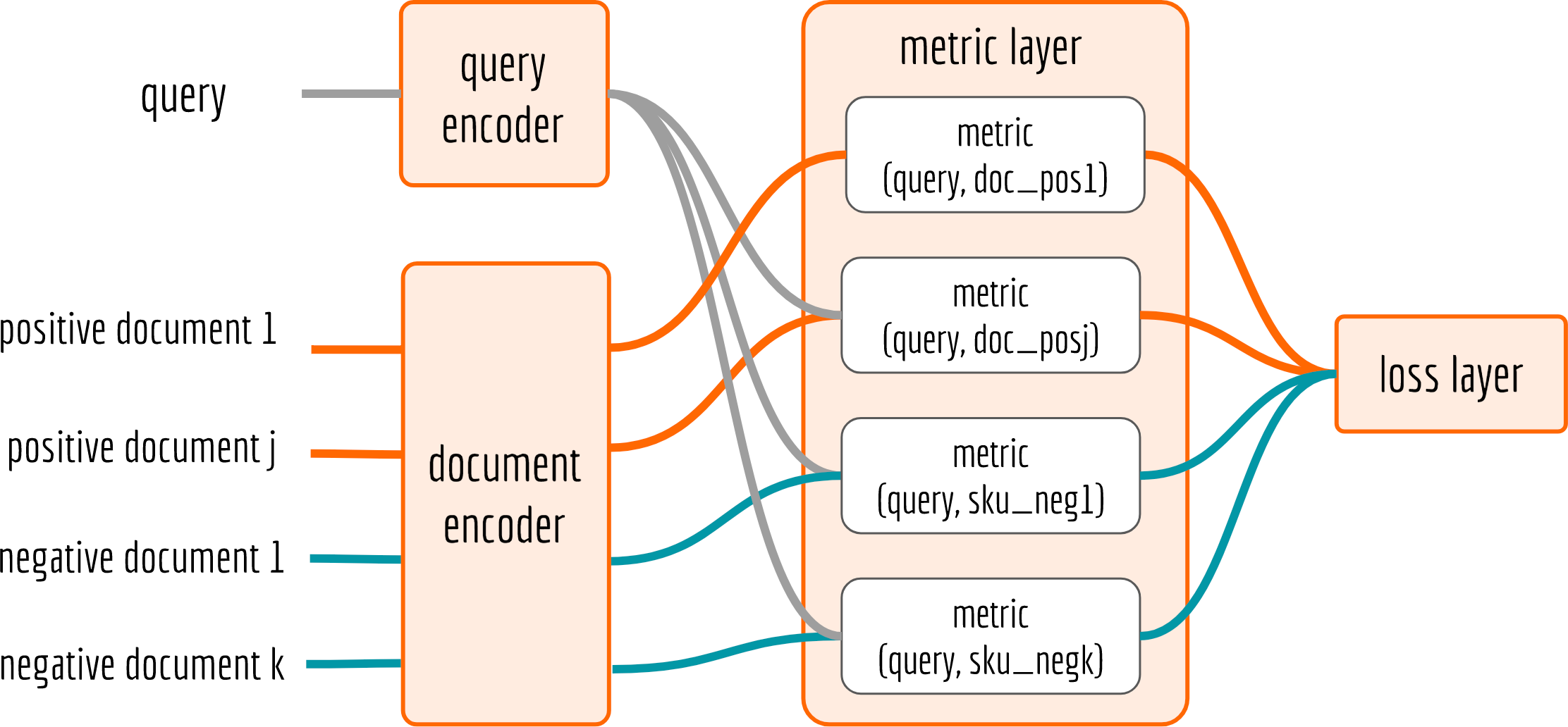
The network has the following structure:

Query and document encoder transform the input to a vector representation, correspondingly. As an example, one can use RNN, LSTM or GRU to encode query and CNN or VAE to encode document/images. The training data is fed from the left. In the next section, I will focus on the implementation of metric layer and loss layer. The encoder and negative sampling are also important to the model performance, but I leave them as a story for another day.
Metric Layer Implementation
The code is fairly straightforward. But one needs to pay attention to the dimension of those tensors.
1 | with tf.variable_scope('Metric_Layer'): |
In the network, variable query is the output from query-encoder, which is in the size of [batch_size, num_hidden]. The document-encoder’s ouput has different size: d_pos_norm is a tensor of [batch_size, num_pos, num_hidden] and d_neg_norm is [batch_size, num_neg, num_hidden]. Therefore, we need to use tf.expand_dims on query to make them size-compatible. For cosine and $\ell_2$ cases, it is unnecessary to tile the tensor as the multiplication and subtraction operations support broadcasting. The figure below explains the data flow when using MLP as the metric.

In the above code, the MLP is implemented as a 64-32-16 feedforward network with softplus activation on each layer.
Loss Layer Implementation
To compute the loss, we must unify the size of metric_p and metric_n. This can be again achieved by using the expand and tile operations on the corresponding axis, as described below. Note that how I expand_dims and tile on different axis for metric_p and metric_n, so that the difference delta can be computed in one-shot.
1 | with tf.variable_scope('Loss_layer'): |
The idea behind is also quite straightforward. First we compute the difference of each triplet (query, positive document, negative document). Then, we feed delta to the loss function and aggregate over all negative documents, via tf.reduce_sum(..., axis=2). Finally we rescale the loss of each query-(postive) document pair by weight and reduce them into a scalar.
Summary
Besides the search, contrastive/rank loss enjoys a wide range of application. One may see it also appears in question-answer, context-aware chatbot and people re-identification tasks. In this article, I showed that such loss generally contains two parts, i.e. the metric and the loss. By leveraging tf.expand_dims, tf.tile and the broadcasting feature of arithmetic operators in Tensorflow, it is fairly straightforward to implement it correctly.