Why I Use raw_rnn Instead of dynamic_rnn in Tensorflow and So Should You
Background
Recently I am working on search queries with Tensorflow. Given an arbitrary query, I am interested in two things: the probability of it and the vector representation of it. After a discussion with my team, I started with a simple generative neural network called Neural Autoregressive Distribution Estimation (NADE), which is designed for modeling the distribution $p(\mathbf{x})$ of input vector $\mathbf{x}$. While I was implementing NADE using dynamic_rnn Tensorflow API, I found it is kind of hacky especially for sampling. Later, I resorted to a low-level API called raw_rnn, which turns out to be more powerful for generative recurrent neural network.
In this article, I want to highlight the advantages of raw_rnn over dynamic_rnn. In particular, I will describe how to use this API to implement NADE and a sequence-to-sequence model. Although raw_rnn is described as a low-level API in the Tensorflow documentation, its usage is quite straightforward. Most importantly, a sampling process implemented by raw_rnn is much more efficient comparing to dynamic_rnn (e.g. this, this and this). It is also easier for debugging. Given that there are not so many articles on the web about using raw_rnn in practice, I hope this article could shed a light on this API and give you some guidance when implementing an RNN next time.
Recap of Neural Autoregressive Distribution Estimation
NADE is one of the most classic generative neural networks developed in 2011. It allows one to model probability density of the input data (i.e. $p(\mathbf{x})$) using neural network. Comparing to nowadays most popular Generative Adversarial Networks (GAN), NADE models the density explicitly in a tractable way.
Formally, let $\mathbf{x}$ be a $D$-dimensional input vector. The distribution $p(\mathbf{x})$ can be factorized as a product of conditional distributions:
$$p(\mathbf{x}) = p(x_1)p(x_2|x_1)\ldots p(x_D|x_{D-1},\ldots, x_1)$$
As you can see, there is a recurrent pattern in the equation above. In fact, this is true for any $D$-dimensional distribution. Given a data set $ \{ \mathbf{x}_{i}\}_{i=1}^{N}$, NADE can be trained by maximizing the likelihood, or equivalently by minimizing the average negative log-likelihood:
$$\frac{1}{N}\sum_{n=1}^N-\log p(\mathbf{x}^{(n)}) =\frac{1}{N} \sum_{n=1}^N\sum_{d=1}^D-\log p(x_d^{(n)}|\mathbf{x}_{<d}^{(n)})$$
Here $\mathbf{x}_{<d}$ contains the first $(d-1)$ dimensions. Depending on the characteristics of the input data $\mathbf{x}$, there are many ways to parametrize those conditional distributions. For example, if your data contains only binary values then Bernoulli distribution is an obivious choice, i.e. $p(x_d|\mathbf{x}_{<d}) = \mathrm{Bernoulli}(p_d)$. For the input data that contains only $k$ discrete values, you may want to use Multinomial distribution, i.e. $p(x_d|\mathbf{x}_{<d}) = \mathrm{Multinomal}(p_{d1},\ldots, p_{dk})$. Of course, different distributions will introduce different number of parameters, e.g. $p_d$ in Bernoulli or $p_{d1},\ldots, p_{dk}$ in Multinomial. Now the remaining task is to model these parameters with some neural network, which will be described in the next section.
NADE-LSTM using raw_rnn
The original NADE paper uses a simple feed-forward network to model the parameter of the distribution. But we don’t have to strictly follow their idea. Here I choose LSTM as the recurrent cell as it doesn’t suffer from the exploding and vanishing gradients problem.
Let’s start with a simple Bernoulli distribution. The following figure depicts the NADE-LSTM network with binary pixel as the input (at the bottom). The pixels on the top are the sampled outputs from the Bernoulli distribution.
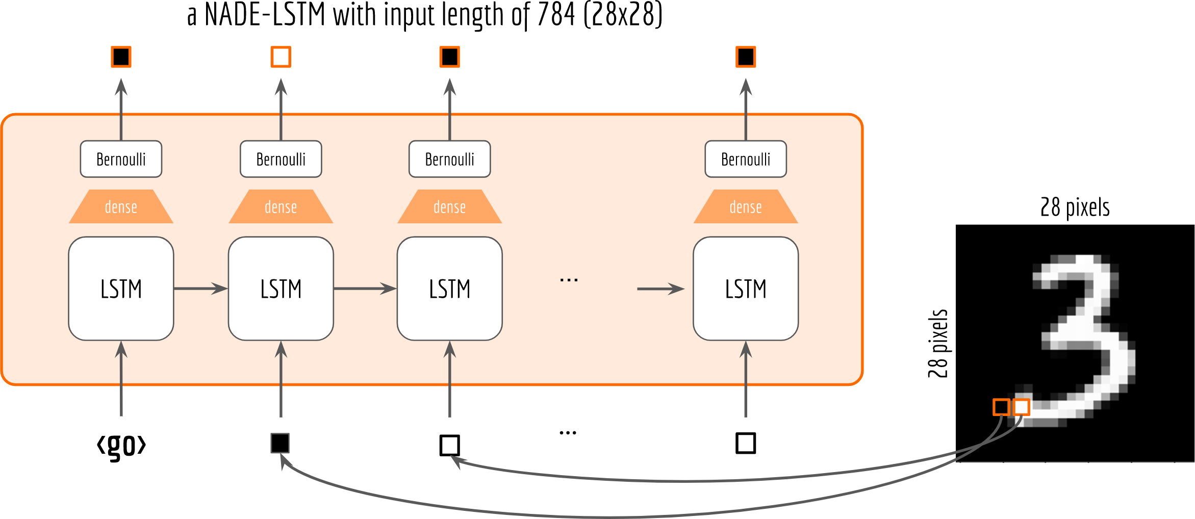
One may observe that, I add a shared dense layer for mapping the LSTM cell’s output to the parameter of the distribution. To make sure that the output of the dense layer is a valid Bernoulli parameter, i.e. $0<p_i<1$, I also put a sigmoid activation on it. This can be done via:
1 | tf.layers.dense(tf.zeros([1, cell.output_size]), units=1, |
Note that although all cells share the same dense layer, their corresponding Bernoulli distributions are not the same due to the information carried on the recurrent structure.
To use raw_rnn to create an RNN, the key is to write your own loop function loop_fn. Generally, you need to clarify these four things in the loop_fn:
- What is the initial state or the input to the cell? (
if cell_output is None:branch) - What is the next state or the next input to the cell? (
elsebranch) - What information do you want to propagate through the network? (
loop_state.write) - When will the recurrence stop? (
elements_finished)
Below is the code for loop_fn in NADE-LSTM, I will explain it in details. I also recommend readers to check the official documentation for reference.1
2
3
4
5
6
7
8
9
10
11
12
13
14
15
16
17
18
19
20
21
22
23
24
25
26output_ta = tf.TensorArray(size=784, dtype=tf.float32) # store trained/sampled pixel
def loop_fn(time, cell_output, cell_state, loop_state):
emit_output = cell_output # == None for time == 0
if cell_output is None:
# time=0, everything here will be used for initialization only
next_cell_state = cell_init_state
next_pixel = cell_init_pixel
next_loop_state = output_ta
else:
# pass the last state to the next
next_cell_state = cell_state
next_pixel = tf.cond(is_training,
                     lambda: inputs_ta.read(time - 1),
                     lambda: tf.contrib.distributions.Bernoulli(
                         probs=tf.nn.sigmoid(tf.layers.dense(cell_output, 1,
                             name='output_to_p', activation=tf.nn.sigmoid,
                             reuse=True)),
                         dtype=tf.float32).sample())
next_loop_state = loop_state.write(time - 1, next_pixel)
elements_finished = (time >= 784)
return (elements_finished, next_pixel, next_cell_state,
emit_output, next_loop_state)
Altering Input to the Cell
One of the biggest advantages of raw_rnn is that you can easily modify the next input to feed to the cell, whereas in dynamic_rnn the input is fixed and usually given the placeholder. This feature is extremely useful when you do sampling. For example, in the code snippet below, I implement the sampling procedure by conditioning on a boolean placeholder is_training:1
2
3
4
5
6
7next_pixel = tf.cond(is_training,
lambda: inputs_ta.read(time - 1),
lambda: tf.contrib.distributions.Bernoulli(
probs=tf.nn.sigmoid(tf.layers.dense(cell_output, 1,
name='output_to_p', activation=tf.nn.sigmoid,
reuse=True)),
dtype=tf.float32).sample())
If is_training is true, then we read from the input placeholder given by feed_dict. Otherwise, we do sampling from a Bernoulli distribution and use the sample as the next input. The following figure visualizes the sampling procedure.
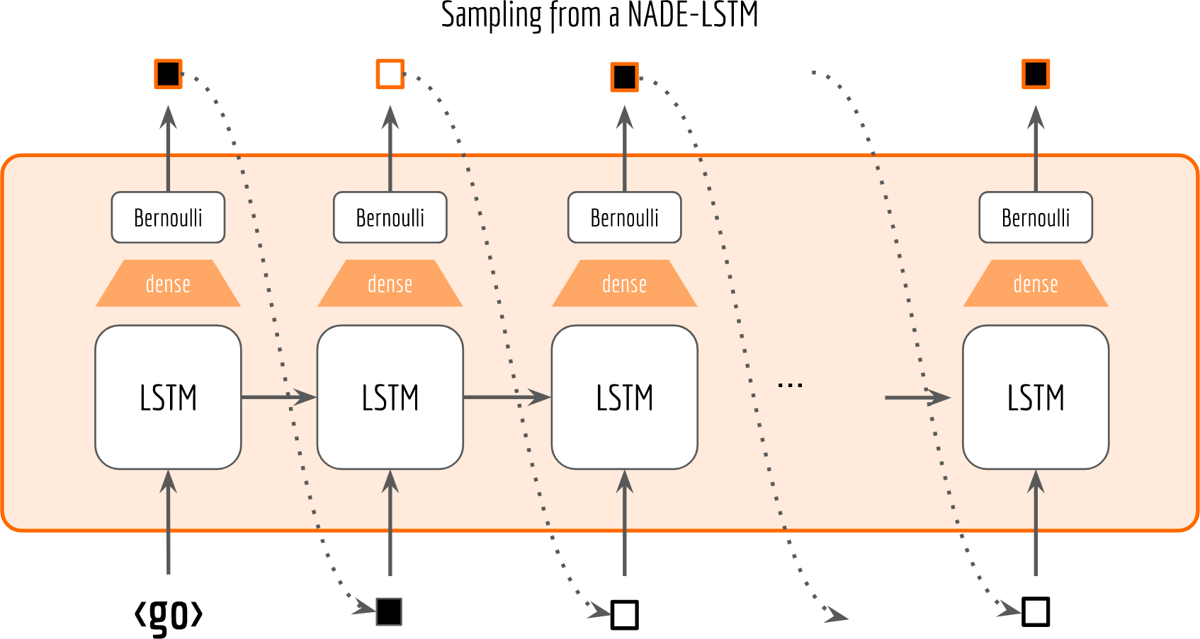
As one can see, with raw_rnn there is no need to adapt or squeeze the graph for sampling. You just set is_training flag to false and that’s it. Moreover, the sampling is highly efficient as you only need to run sess.run once. Comparing to the most Tensorflow sampling implementations you can find on the web (e.g. this, this and this), they are roughly based on the following pattern:1
2
3
4
5
6samples = []
for i in range(max_time):
new_input = update_feed_dict(current_input, new_state)
preds, new_state = sess.run([node_sample, node_final_state],
feed_dict=new_input)
samples.append(preds)
, where max_time is the length of the sampled sequence. On MNIST data set, max_time is 784. The problem of this code is that it will call sess.run() max_time times, whereas each time only with a tiny job. If your graph computation is on GPU, then frequently alternating the context between CPU and GPU is inefficient especially when max_time is large.
Here is another usage. Say if we want to learn the conditional density of pixels given class labels, i.e. $p(\mathbf{x}|y)$, where $y\in \{ 0, 1, \ldots, 9 \} $. We can simply let Y be a tf.placeholder and add the following line at the end of loop_fn scope:
1
next_pixel = tf.concat([next_pixel, Y], axis=1)
Isn’t that much simpler than adding/changing nodes in computation graph?
Propagate Information through RNN Loop
With raw_rnn you can propagate any information through the loop, or send it out to feed your downstream nodes. In the aforementioned NADE-LSTM example, I’m interested in what the network samples at each step, i.e. next_pixel drawed from the Bernoulli distribution. This is how I store it:1
2
3
4
5
6
7
8
9output_ta = tf.TensorArray(size=784, dtype=tf.float32) # store sampled pixels
def loop_fn(time, cell_output, cell_state, loop_state):
if cell_output is None:
#...
next_loop_state = output_ta
else:
#...
next_loop_state = loop_state.write(time - 1, next_pixel)
#...
To read output_ta from an RNN:1
2
3from tensorflow.python.ops.rnn import _transpose_batch_time
_, _, loop_state_ta = tf.nn.raw_rnn(LSTMCell, loop_fn)
X_sampled = _transpose_batch_time(loop_state_ta.stack())
Note that loop_state_ta is a TensorArray and is in [time, batch, input_depth] shape. Therefore you need to first stack() it to make it a Tensor. Then transpose the batch and time dimensions of it to make it consistent with your input format.
What if I want to write more information at each step? No problem. Just make output_ta a tuple of TensorArray. Here is an example:1
2
3
4
5
6
7output_ta = (tf.TensorArray(size=784, dtype=tf.float32), # save sampled pixels
tf.TensorArray(size=784, dtype=tf.float32)) # save model loss
def loop_fn(time, cell_output, cell_state, loop_state):
#...
next_loop_state = (loop_state[0].write(time - 1, next_pixel),
loop_state[1].write(time - 1, logp_loss(cell_output, next_pixel)
if save_memory else 1))
In the code above, I write the next pixel as well as the aggregated log-probability loss to output_ta at each time step. One may argue that a more time-efficient way is to concatenate the whole sequence of the cell outputs in time, and then compute the loss on this batch-concatenated sequence. However, when the sequence is very long and the number of hidden units of the cell is large, such method won’t work due to the GPU memory limit. Imagine we use a LSTM with 512 hidden units on MNIST data (784-dim) and set with size of the batch to 400, then the overall output from the network will be a [400, 512, 784] float32 Tensor, about 0.64 GB of memory. And did I mention you need to run it for validation set as well (which is often much bigger than 400)? In the example above, I use a boolean flag save_memory. If it is set to true, then I only keep a scalar value for the loss each time step and reduce them afterwards. This allows me to switch between a quick test (e.g. local debugging) and some real deals with big data and large network.
For those who are interested in details inside the RNN loop, and for those who simply want to debug by inspecting intermediate values, raw_rnn gives an elegant solution.
Now let’s have some fun. I do sampling after every epoch and check how NADE-LSTM captures the density of input pixels. Remember, all you need is letting is_training=False. Here is how it looks like:
Without any modification on the algorithm, let’s apply it to Fashion-MNIST dataset, which is a direct drop-in replacement for the original MNIST.
Results are not as good as the original MNIST. But that’s fine. After all, NADE is a simple autoregressive model. Besides, Fashion-MNIST is more challenging than the original MNIST.
A Sequence-to-Sequence Model for Query Embedding
Before I wrap up this article, I want to give another example of a sequence-to-sequence model for query embedding. In this example, I will use both dynamic_rnn and raw_rnn to build the network, which nicely leverages the simplicity of dynamic_rnn and the flexibility of raw_rnn. If you are not familiar with the sequence-to-sequence model, I highly recommend you to read this paper. If you already understand what I wrote in the previous sections, then please consider this as a small exercise.
Let’s start by drawing the architecture first.
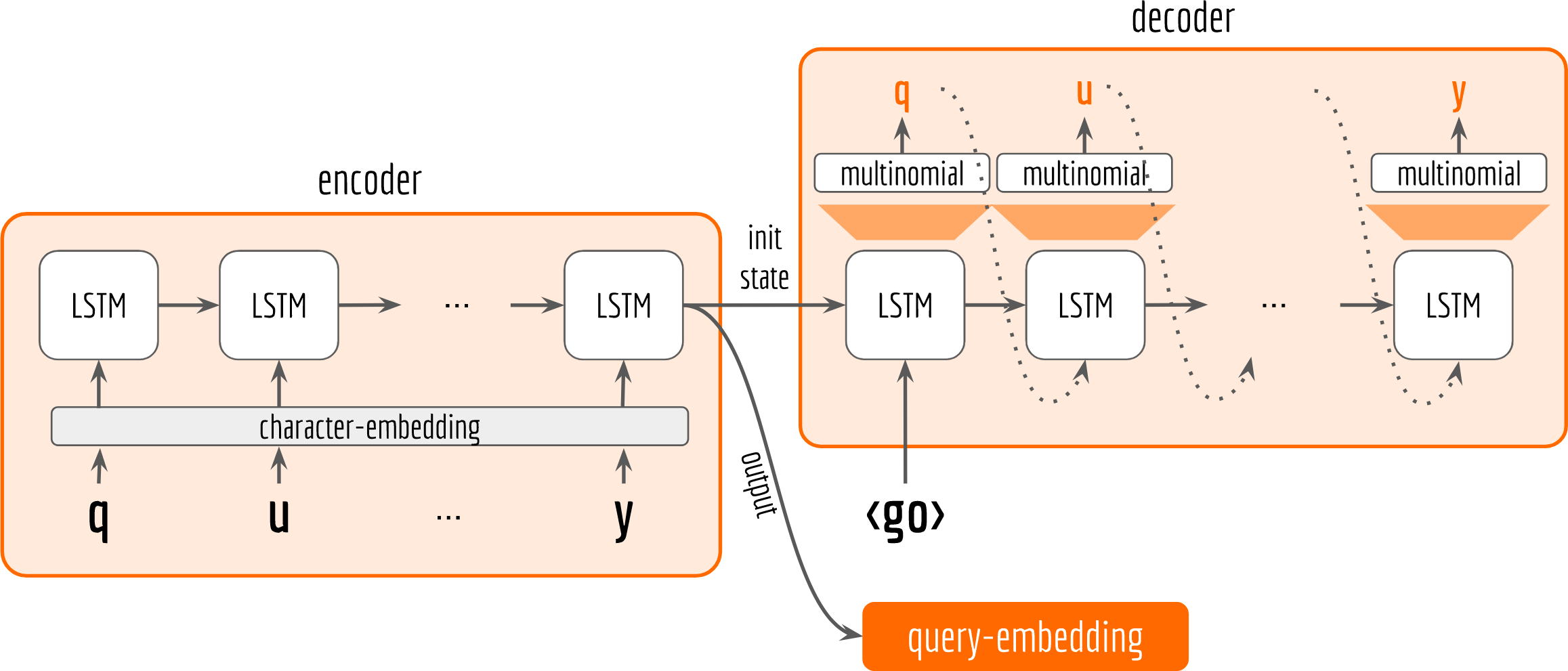
In general, our architecture follows the encoder-decoder pattern. Both encoder and decoder are character-based LSTM. The encoder observes the training data and receives input character by character. The last state from encoder is then fed to the decoder as initial state. The decoder does not observe the training data. It only receives the encoder’s last output and state. Inside the loop of decoder, it keeps sampling and use the sample as next input to the LSTM cell. The network’s parameters are optimized by making the sampled sequence (orange letters in the decoder box) close to the input sequence (black letters in the encoder box), which can be quantified with sigmoid cross-entropy loss. Finally, the last output from encoder is used as our query embedding.
There is nothing really special about the encoder, thus I use dynamic_rnn to implement it:1
2
3
4
5
6
7with tf.variable_scope('Encoder'):
encoder_outputs, last_enc_state = tf.nn.dynamic_rnn(LSTMCell,
inputs=X_embd,
sequence_length=L,
dtype=tf.float32)
with tf.variable_scope('Query_Embedding'):
query_embedding = get_last_output(encoder_outputs, L, 'embedding_vector')
Here X_embd is the one-hot embedding for the input characters and L is a [batch_size] Tensor represents the length of each sequence in the batch.
For sampling and feeding the sample to the cell in the decoder, I use raw_rnn:1
2
3
4
5
6
7
8
9
10
11
12
13
14
15
16
17
18
19
20
21
22
23
24
25
26
27
28with tf.variable_scope('Decoder'):
with tf.variable_scope('Initial_GO_Input'):
dummy_zero_input = tf.zeros(shape=[cur_batch_size,
cur_batch_depth], dtype=tf.float32,
name='dummy_zero_input')
output_ta = tf.TensorArray(size=cur_batch_time, dtype=tf.int32)
def loop_fn(time, cell_output, cell_state, loop_state):
emit_output = cell_output # == None for time == 0
if cell_output is None:
next_cell_state = last_enc_state
next_sampled_onehot = dummy_zero_input
next_loop_state = output_ta
else: # pass the last state to the next
next_cell_state = cell_state
next_sampled_input = get_sample(cell_output) # sampling from multinomial
next_sampled_onehot = tf.nn.embedding_lookup(embeddings, next_sampled_input)
next_loop_state = loop_state.write(time - 1, next_sampled_input)
elements_finished = (time >= cur_batch_time)
next_input = next_sampled_onehot
return (elements_finished, next_input, next_cell_state, emit_output, next_loop_state)
decoder_emit_ta, _, loop_state_ta = tf.nn.raw_rnn(LSTMCell, loop_fn)
In get_sample, I use tf.distributions.Categorical.sample to draw from cell-specific multinomial distribution, which is parametrized by a dense layer of size [num_hidden_units, num_chars]. get_sample returns an integer Tensor representing int-indexed characters. This is very useful for me to visually check what the network is decoding, so I stroe it in loop_state and send it out at the end of the loop. On the other hand, the LSTM cell needs a vector representation as input. Thus, I transform the sample to one-hot embedding with embedding_lookup and use as next input to the cell.
Now let’s build the loss function and some metrics.1
2
3
4
5
6
7
8
9with tf.name_scope('Output'):
decoder_emits = _transpose_batch_time(decoder_emit_ta.stack())
logits = get_logits(decoder_emits)
X_sampled_int = _transpose_batch_time(loop_state_ta.stack())
with tf.name_scope('Decoder_Loss'):
logp_loss = -tf.reduce_mean(tf.log(1e-6 + get_prob(decoder_emits, X)))
xentropy_loss = tf.reduce_mean(tf.nn.sigmoid_cross_entropy_with_logits(labels=X_embd, logits=logits))
sampled_acc = tf.reduce_mean(tf.cast(tf.equal(X, X_sampled_int), tf.float32))
Readers may notice that this time I compute the loss function outside the loop_fn unlike what I wrote in the last section. This is because query sequences are short in general, much shorter than 784 (i.e. the MNIST dimensions) at least. In this case, computing the loss in batch gives better efficiency.
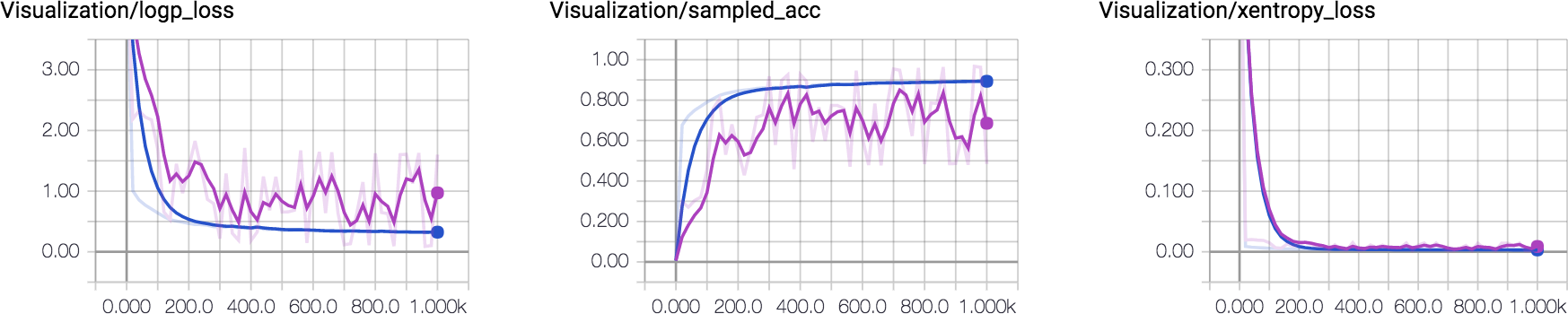
Finally, you can choose your favorite optimizer and minimizing xentropy_loss or logp_loss. For visualizing the training progress in a more intuitive way, I add sampled_acc for measuring the accuracy of sampled sequence.
I plot how these metrics change over time. One can observe that the sampled accuracy for training and validation set converge to 80%~90% eventually. This was made using LSTM with 64 hidden units. Increasing the capacity of LSTM would yield better accuracy.
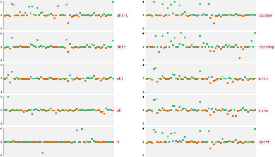
Now who wants to see the how the query embedding look like? In the following figures, I plot the 64-dimensional query embedding with blue and red points. Green points represent positive values, reds are negative. All values are in [-1, +1]. Note how embedding is robust to the misspelled words, and how it changes while I typing.
Pitfalls of raw_rnn
raw_rnnuses TensorArray for the input and outputs, in which Tensor must be in [time, batch_size, input_depth] shape. This is different from the shape we are familiar with, i.e. [batch_size, time, input_depth]. So don’t forget to transform your input into the correct format before feeding it toraw_rnn:1
2inputs_ta = tf.TensorArray(size=cur_batch_time, dtype=tf.float32).unstack(
_transpose_batch_time(self.input), 'TBD_Input')And transform it back when you read the output:
1
rnn_outputs = _transpose_batch_time(rnn_output_ta.stack())
When you alter
next_inputinside theloop_fn, Tensorflow may lose the track for back-propagating the gradient. Consequently, you will receive the following warning:In this case, just add
UserWarning: Converting sparse IndexedSlices to a dense Tensor of unknown shape. This may consume a large amount of memory.
“Converting sparse IndexedSlices to a dense Tensor of unknown shape. “stop_gradientto stop gradient propagating through your input, like this:1
2
3next_pixel = tf.stop_gradient(tf.cond(is_training,
lambda: inputs_ta.read(time - 1),
lambda: get_sample(cell_output)))
Conclusion
To summarize, raw_rnn provides you the flexibility to customize recurrent neural network and helps you understand the recurrence mechanism better. It allows you to control what should output, what should be fed next, and when should it end. This is extremely useful when you want to design sophisticated recurrent neural network. I hope this article could shed a light on this useful API and bring your RNN to the next level.