Teach Machine to Comprehend Text and Answer Question with Tensorflow - Part I
Background
The part II of this series is avaliable now, in which I present a unified model for asking and answering!
Reading comprehension is one of the fundamental skills for human, which one must learn systematically since the elementary school. Do you still remember how the worksheet of your reading class looks like? It usually consists of an article and few questions about its content. To answer these questions, you need to first gather information by collecting answer-related sentences from the article. Sometimes you can directly copy those original sentences from the article as the final answer. This is a trivial “gut question”, and every student likes it. Unfortunately (for students), quite often you need to summarize, assert, infer, refine those evidences and finally write the answer in your own words. Drawing inferences about the writer’s intention is especially hard. Back in high school, I was often confused by the questions like “why did the poet write a sentence like this?” How could I possibly know the original intention of an ancient poet a thousand years ago? How could my teacher know it for sure?
Now at Tencent AI Lab, I’m leading a team teaching machines to comprehend text and answer questions as we did in schools. Why is it interesting to us? Because I believe the ability to comprehend text will lead us to a better search.
Considering your journey with a traditional keyword-based search. You have a question in mind and hope the internet can answer you. As a start, you formulate the question with some keywords and type them into the search box. The search engine returns a set of matched documents. Then, you pick top-ranked documents and quickly scan them through, as the answer to the question often hides somewhere in those documents. Finally, you marry multiple ideas from various texts and draw a conclusion about the answer. Note that in this journey, the search engine only helps you filtering out irrelevant documents, leaving the hard tasks such as reading, comprehending and summarizing to yourself. Though the “highlighting” feature of some search engines allows you to quicker locate related passages (n.b. related to the question not to the potential answer, these are different), you still have to identify them and make inference. In other word, the mighty internet doesn’t actually answer your question, you answer it by yourself! The next picture illustrates this process.
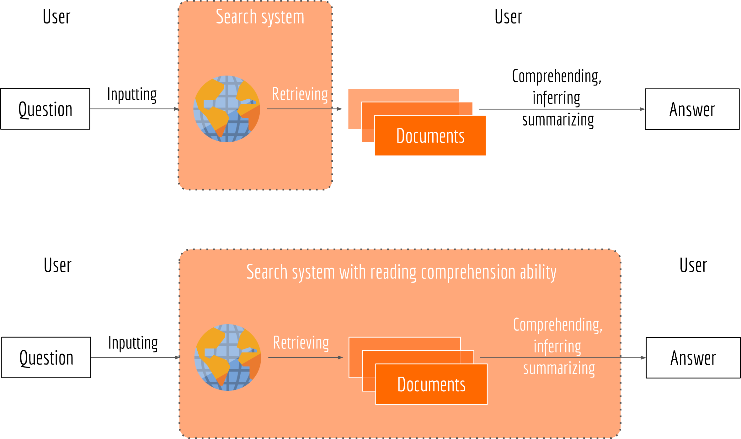
Having a search system with the reading comprehension ability can make the user experience smoother and more efficient, as all time-consuming tasks such as retrieving, inferring and summarizing are left to the computers. For impatient users who don’t have time to read text carefully, such system can be very useful. For machine learning developers, such system is challenging. An algorithm that returns query-relevant documents is far from enough. The algorithm should also have the abilities to follow organization of document, to draw inferences from a passage about its contents, and to answer questions answered in a passage.
In this article, I will describe how to implement a reading comprehension system from scratch using Tensorflow. This article is the first part of the reading comprehension series I planed. This first part serves as a tutorial of machine reading comprehension. I will define the problem, propose a general neuron network structure for this task, and try my best to help you understand this challenge. In the second part (not published yet), I will discuss more sophisticated network structures and technical details which are required for building a production-level reading comprehension system.
Table of Content
- Problem Definition
- Network Architecture
- Embedding and Encoding Layers
- Matching Layer
- Fusing Layer
- Decoding Layer & Loss Function
- Predicting the Answer Span
- Moving Forward to Part II
Problem Definition
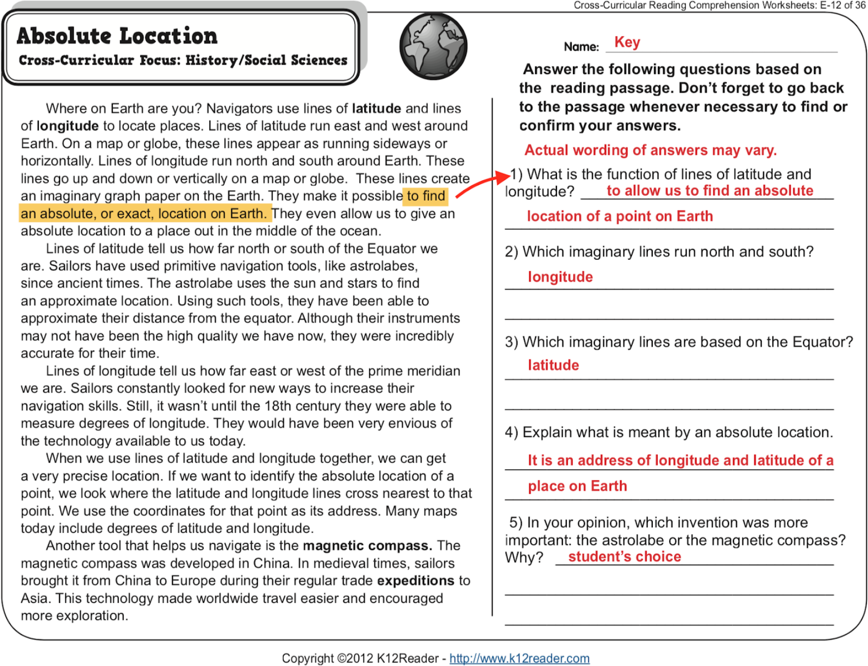
Given a question $q \in \mathcal{Q}$, let’s start by assuming a search engine already provides us a set of relevant passages $P=\{p_1,\ldots,p_M \,|\, p_i \in \mathcal{P}\}$ (e.g. using symbolic matching). Each passage $p_i$ consists of few sentences, as illustrated in the “Absolute Location” worksheet above. Note that the answer to $q$ may not be a complete passage or a sentence. It can be a subsequence of a sentence, or a sequence spans over multiple sentences or passages. Without lose of generality, we define two finite integers $s, e\in [0, L)$ to represent the start and end position of the answer, respectively. Here $L$ denotes the total number of tokens of the given passage set. Of course, a valid answer span also requires $e > s$.
Consequently, our training data can be represented as $\mathcal{T}=\{q_i, P_i, (s, e)_i\}_{i=1}^{N}$. Given $\mathcal{T}$ the problem of reading comprehension becomes: finding a function $f: \mathcal{Q}\times\mathcal{P}\rightarrow\mathbb{Z}^2$ which maps a question and a set of passage from their original space (i.e. $\mathcal{P}$ and $\mathcal{Q}$, respectively) to a two-dimensional integer space. To measure the effectiveness of $f$, we also need a loss function $\ell:\mathbb{Z}^2\times\mathbb{Z}^2\rightarrow\mathbb{R}$ to compare the prediction with the groundtruth $(s, e)_i$. The optimal solution $f^{*}$ is defined as
$$f^{*} := \arg\min_f \sum_{i=1}^N\ell\Bigl(f(q_i, \mathcal{P}_i), (s, e)_i\Bigr).$$
Careful readers may now have plenty of questions in mind:
- What is the exact form of function $f$?
- How to represent question and passage in the vector space?
- What is a good loss function?
- What if an answer contains multiple non-consecutive sequences?
- What if an answer must be synthesized rather than extracted from the context, e.g. the 5th question in our first “Absolute Location” worksheet?
It is not surprising that I choose deep neuron network to model $f$, as $f$ needs to be complicated enough to capture the deep semantic correlation between passages and questions. I will unfold the remaining parts of this post to answer the aforementioned questions.
Network Architecture
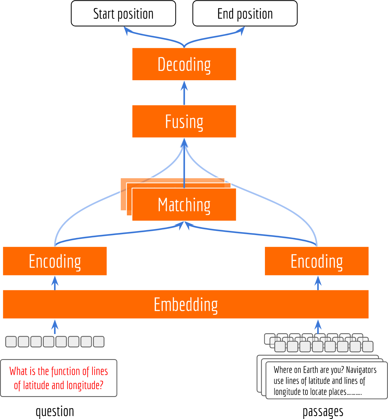
The next picture illustrates an overview of a reading comprehension network. From bottom up there are five layers in this network: embedding layer, encoding layer, matching layer, fusion layer and decoding layer. The input to the network are tokens of a question and the corresponding passages. The output from the network are two integers, representing the start and end positions of the answer. Note that the choice of the model is quite open for all layers. For the sake of clarity, I will keep the model as simple as possible and briefly go through each layer.
Embedding and Encoding Layers
The embedding and encoding layers take in a sequence of tokens and represent it as a sequence of vectors. Here I implement them using a pretrained embedding matrix and bi-directional GRUs. To load a pretrained embedding into the graph:
1 | embed_shape = [vocab_size, vocab_embed_dim] |
Note that the embedding matrix is initialized only once and not trained in the entire learning process. If you work with a language with a large vocabulary, the embedding matrix would be so big that almost all parameters of the model come from the embedding matrix. Therefore, fixing the embedding can often improve the effectiveness of training.
Encoding question and passage sequence with bidirectional GRU is straightforward using Tensorflow API.1
2
3
4
5
6
7
8
9
10
11q_emb = tf.nn.embedding_lookup(word_embed, q)
with tf.variable_scope('Question_Encoder'):
cell_fw = GRUCell(num_units=hidden_size)
cell_bw = GRUCell(num_units=hidden_size)
output, _ = tf.nn.bidirectional_dynamic_rnn(cell_fw, cell_bw, q_emb, sequence_length=q_len)
# concat the forward and backward encoded information
q_encodes = tf.concat(output, 2)
# do the same to get `p_encodes`
The choice of the cell is quite open. For example, GRUCell can be wrapped with DropoutWrapper and MultiRNNCell to get stabler and richer representations. Alternatively, one can share the parameters of the passage encoder and the question encoder to reduce the model size. However, this comes with a cost of less effective training.
Matching Layer
Now that we have represented questions and passages into vectors, we need a way to exploit their correlation. Intuitively, not all words are equally useful for answering the question. Therefore, the sequence of passage vectors need to be weighted according to their relations to the question. The next picture illustrates this idea.
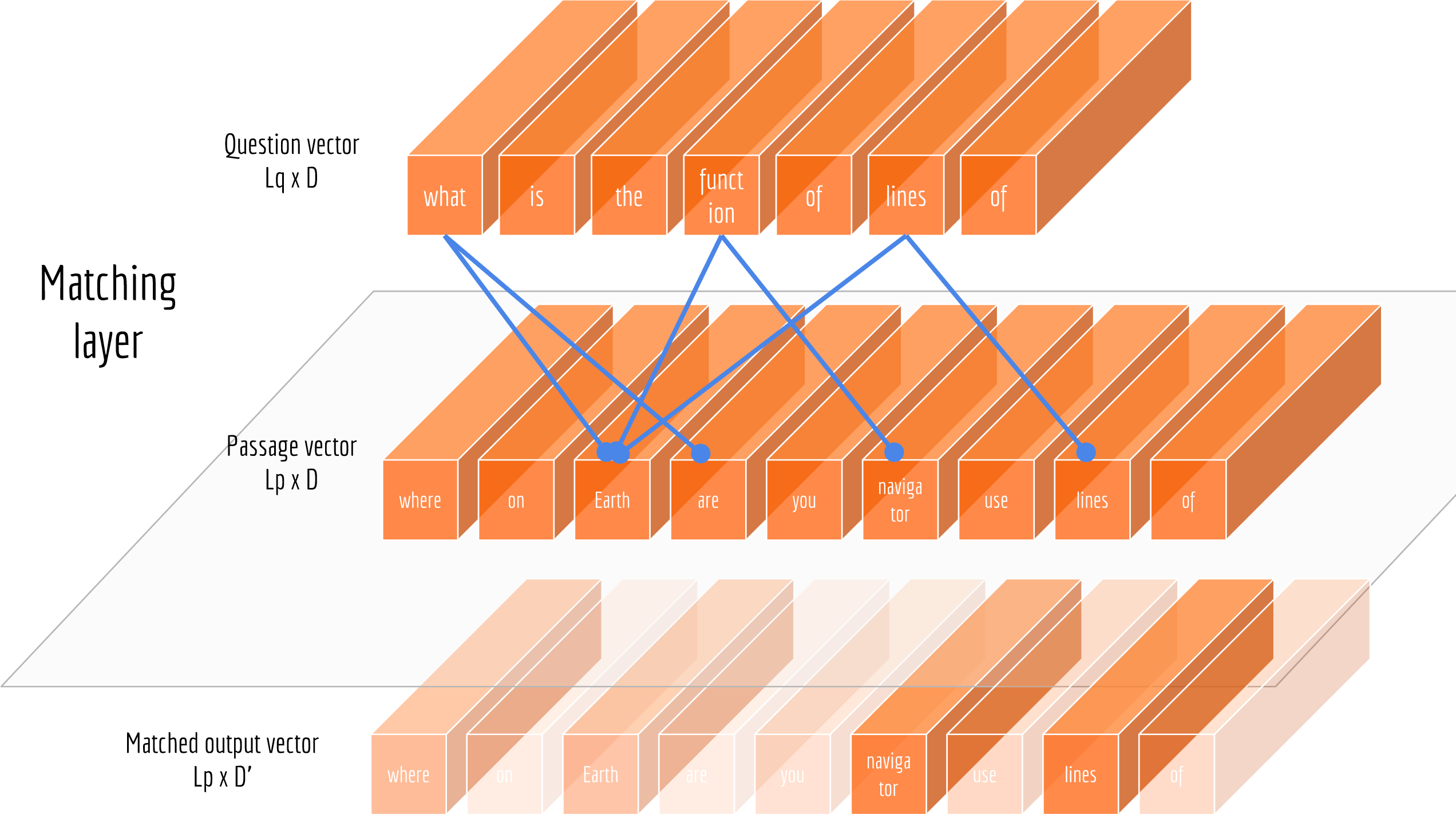
Attention mechanism is one of the most popular methods to solve this problem. Here I want to introduce an interesting method used in the paper “Bi-Directional Attention Flow for Machine Comprehension”. The idea is to compute attentions in two directions: from passage to question as well as from question to passage. Both of these attentions are derived from a shared similarity matrix $\mathbf{S}$, in which each element $s_{ij}$ represents the similarity between the $i$th token of the passage and the $j$th token of the question. If we denote the similarity function as $k: \mathbb{R}^D\times\mathbb{R}^D\rightarrow\mathbb{R}$, then each element in $\mathbf{S}$ can be represented as:
$$s_{ij}=k(\mathbf{p}_{:i}, \mathbf{q}_{:j}).$$
If you come from the pre-deep learning era, then you should be very familiar with the above equation. This old friend is exactly the kernel function used in support vector machines and Gaussian process! Thus, I can also employ RBF kernel, polynomial kernel here for the same purpose. The code below shows a very simple version with a fixed linear kernel. Curious readers are recommended to read Section 2.4 “Attention Flow Layer” of this paper for more sophisticated “kernel” functions.
1 | p_mask = tf.sequence_mask(p_len, tf.shape(p)[1], dtype=tf.float32, name='passage_mask') |
Three remarks about this implementation. First, as the length of questions/passages is vary inside each batch, one has to mask out the padded tokens from the calculation to get correct gradient. Since I’m using softmax to normalize the similarity score, the correct way to mask out padded element is to subtract a negative number with large magnitude before doing softmax.
Second, match_out at the last step consists of the original passage encoding and two weighted passage encodings. Concatenating the output from the previous encoding layer can often reduce the information loss caused by the early summarization.
Finally, note that the first two dimensions of match_out is the same as the p_encodes from the encoding layer. They only differ in the last dimension, i.e. depth. As a consequence, one may consider match_out as a passage encoding conditioned on the given question, whereas p_encodes captures the interaction among passage tokens independent of the question.
Fusing Layer
The fusing layer is designed with two purposes. First, capturing the long-term dependencies of match_out. Second, collecting all the evidences so far and preparing for the final decoding. A simple solution would be feeding match_out to a bi-directional RNN. The output of this RNN is then the output of the fusing layer. This implementation looks very similar to our encoding layer described above. Unfortunately, such method is not very efficient in practice, as RNN is generally difficult to parallelize for GPU. Alternatively, I use CNN here to capture long-term dependencies and summarize high-level information. Specifically, I employ (multiple) conv1d layer(s) to cross-correlated with match_out to produce the the output of the fusing layer. The next figure illustrates this idea.
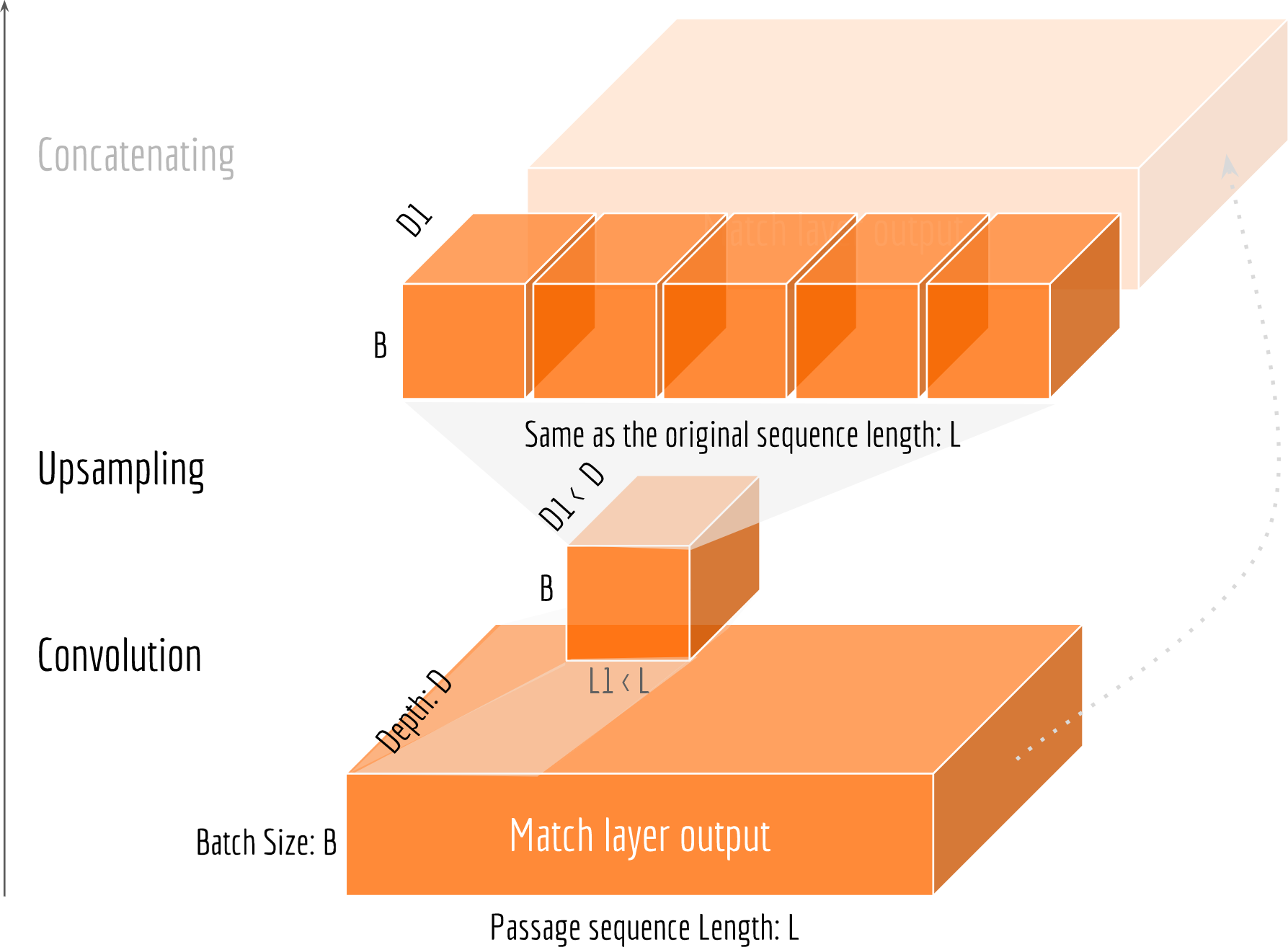
1 | out_dim = 64 |
The upsampling step is required for concatenating the convoluted features with match_out and p_encodes. It can be implemented with resize_images from Tensorflow API. The size of fuse_out is [B,L,D], where B is the batch size; L is the passage length and D is the depth controlled by the convolution filters in the fusing layer.
Decoding Layer & Loss Function
Our final step is to decode fuse_out as an answer span. In particular, here I decode the fused tensor into two discrete distributions $\widehat{\mathbf{s}}$, $\widehat{\mathbf{e}}$ over $[0, L)$, which represent the start and end probability on every position of a $L$-length passage, respectively. A simple way to get such distribution is to reduce the last dimension of fuse_out to 1 using a dense layer, and then put a softmax over its output.
Having now two labels $s, e\in[0,L)$ and two predicted distributions $\widehat{\mathbf{s}}$, $\widehat{\mathbf{e}}$ over $[0, L)$, the training loss can be easily measured using the cross-entropy function. The code below shows how to decode an answer span and compute its loss in Tensorflow.1
2
3
4
5
6
7
8
9
10
11start_logit = tf.layers.dense(fuse_out, 1)
end_logit = tf.layers.dense(fuse_out, 1)
# mask out those padded symbols before softmax
start_logit -= (1 - p_mask) * 1e30
end_logit -= (1 - p_mask) * 1e30
# compute the loss
start_loss = tf.losses.sparse_softmax_cross_entropy(labels=start_label, logit=start_logit)
end_loss = tf.losses.sparse_softmax_cross_entropy(labels=end_label, logit=end_logit)
loss = (start_loss + end_loss) / 2
Careful readers may realize that I have transformed the original integer prediction problem to a multi-class classification problem. I’m not cheating. In fact, this is one popular way to design the decoder. However, there are some underlying problems of this approach:
- The
start_logitandend_logitare decoded separately, whereas intuitively one expects that the end position depends on the start position. - The loss function is not position-aware. Say the groundtruth of the start position is
5, the penalty of decoding it to100would be the same as decoding it to6, even though6is a much better shot.
Let’s keep those questions and curiosity in mind, I will discuss about the solution in the second part of this series.
Predicting the Answer Span
With the start and end distributions $\widehat{\mathbf{s}}$, $\widehat{\mathbf{e}}$ over $[0, L)$, we can compute the probabilities of all answer spans using the outer product of $\widehat{\mathbf{s}}$ and $\widehat{\mathbf{e}}$. Say your total passage length $L$ is 2000, computing $\widehat{\mathbf{s}}\otimes\widehat{\mathbf{e}}$ gives you a [2000, 2000] matrix, of which each element represents the probability of an answer span. The solution space looks pretty huge at the first glance, fortunately not all solutions from this space are valid when you think about it. In fact, the number of effective solutions is much smaller than 4 million as we shall see.
The reason is that a valid solution must satisfy the constraint of $s$ and $e$. First, $e$ must be greater than $s$, filtering out the lower part of the solution matrix. Second, the answer length $e-s +1$ is often restricted in practice: a good answer should not concise and not too long; it should also not across over sentences, etc. This suggests that a valid solution must be in the central band of the matrix. The next picture illustrates this idea.
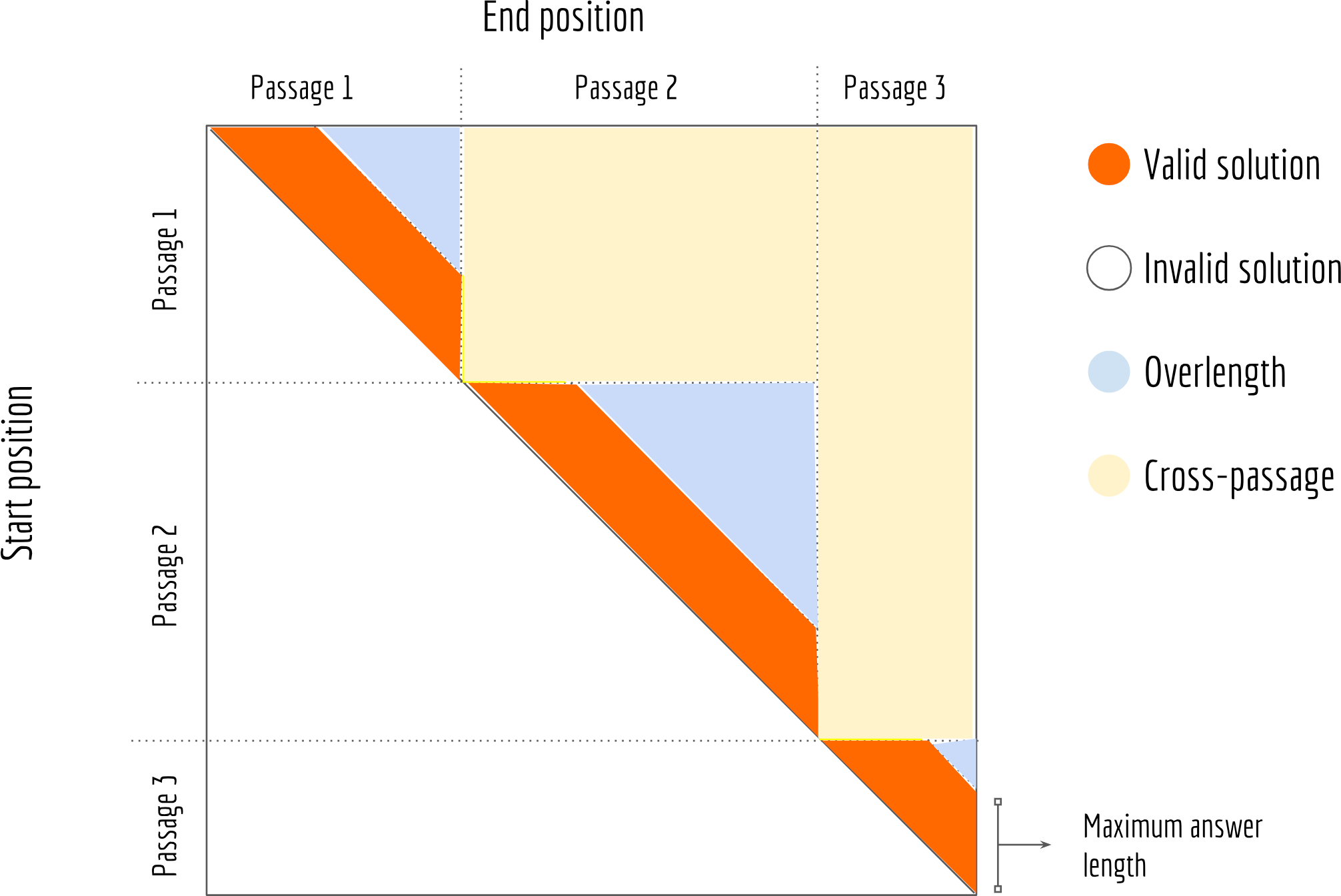
The optimal solution corresponds to the maximum element in the orange band, whose row-index is the start position and column-index is the end position. The code below shows how to implement it with Tensorflow.
1 | # set the maximum answer length |
Moving Forward to Part II
Machine Reading Comprehension enables computers to understand human language. It is considered as one of the core abilities of artificial intelligence. A good reading comprehension system is a great value for industry applications such as search engines. In this article, I have introduced machine reading comprehension challenge and described a simple network to tackle this challenge. In the second part of this series, we will go through each layer to examine its limitation and replace it with a more sophisticated network structure. See you soon!