Serving Google BERT in Production using Tensorflow and ZeroMQ

This is a post explaining the design philosphy behind my open-source project bert-as-service, a highly-scalable sentence encoding service based on Google BERT and ZeroMQ. It allows one to map a variable-length sentence to a fixed-length vector. In case you haven’t checked it out yet, https://github.com/hanxiao/bert-as-service

Background

When we look back at 2018, one of the biggest news in the world of ML and NLP is Google’s Bidirectional Encoder Representations from Transformers, aka BERT. BERT is a method of pre-training language representations which achieves not only state-of-the-art but record-breaking results on a wide array of NLP tasks, such as machine reading comprehension.

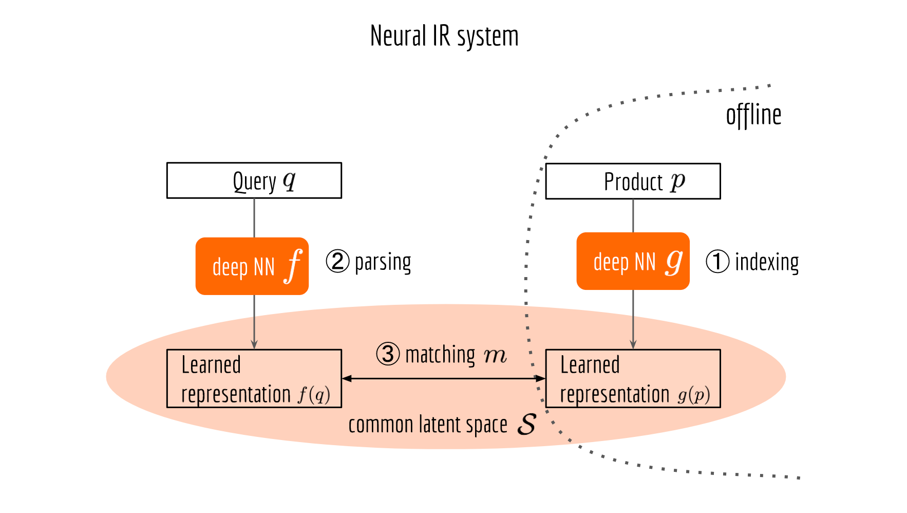
To my team at Tencent AI Lab, BERT is particularly interesting as it provides a novel way to represent the semantic of text using real-valued fixed-length vectors. For many real-world NLP/AI applications that we are working on, an effective vector representation is the cornerstone. For example in the neural information retrieval, query and document need to be mapped to the same vector space, so that their relatedness can be computed using a metric defined in this space, e.g. Euclidean or cosine distance. The effectiveness of the representation directly determines the quality of the search.

So if many NLP applications rely on semantic features, then why don’t we build a sentence encoding infrastructure that can serve multiple teams? This idea, despite how simple and straightforward, is not really practical until recently. Because many deep learning algorithms tailor the vector representation to a specific task or domain. Consequently, the representation from one application/team is not really reusable to other applications/teams. On contrary, BERT (as well as ELMo and ULMFit) decomposes an NLP task into task-independent pretraining and task-specific fine-tuning stages, where pretraining learns a model that is general enough and can be reused in many downstream tasks.

Over the past few weeks, I implemented this idea as an open-source project bert-as-service. It wraps the BERT model as a sentence encoding service, allowing one to map a variable-length sentence to a fixed-length vector. It is optimized for inference speed, low memory footprint, and scalability. The README.md and documentation already cover the usage and APIs very well. In this article, I will focus on the technical details especially the design philosophy about this project, which I hope can offer you some references when serving a Tensorflow model in production.

• BERT Recap
• BERT as a service
• Research: Finding an Effective Embedding/Encoding
• Engineering: Building a Scalable Service
  • Decoupling BERT and downstream network
  • Serving with fast inference speed
  • Serving with low latency
  • Serving with high scalability
• Summary

BERT Recap

There are several highlights in BERT: multi-head self-attention network, dual training task (i.e. masked language model and next sentence prediction), large-scale TPU training. All these features together make this record-breaking NLP model. But good performance is just one part of the story. What I like the most is the design pattern of BERT: it trains a general-purpose “language understanding” model on a large text corpus (e.g. Wikipedia), and then uses that model for a variety of NLP tasks that we care about. Unlike the end-to-end learning, BERT decomposes a traditional NLP learning task into two stages: pretraining and fine-tuning:

• Pretraining learns from plain text data that is publicly available on the web, with the goal of capturing the general grammar and contextual information of a language.
• Fine-tuning learns from a specific task (e.g. sentiment analysis, machine translation, reading comprehension) or data from a particular domain (e.g. legal documents).

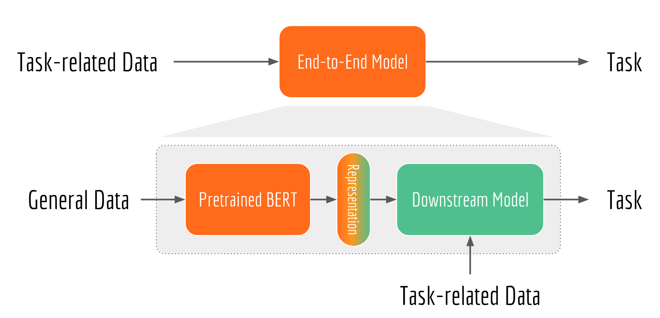
However, pretraining is a time-consuming procedure which requires a lot of computational resources. According to Google, it took them four days on 4 to 16 Cloud TPUs to finish the pretraining. This is way beyond the patience of most researchers and engineers (and of course product owners). Fortunately, this is a one-time thing for every language, and Google has released pretrained BERT models for multiple languages. In practice, you can simply download a pretrained BERT, feed its output representation to a downstream network customized to your task. Note, as the general language information has been already memorized in the pretrained BERT, a light-weight downstream network is often quite sufficient. You may also fine-tune the complete network (i.e. BERT + downstream network) in an end-to-end manner.

BERT as a service

What do we actually want from a BERT model? In the IR/search domain, we want the vector representation of query and document, using it to compute similarity or relatedness between query and document. In the classification-oriented tasks, we want to use the vector representations as well as the pre-annotated labels to train a downstream classifier. In the ensemble learning system, we want the BERT vector as a part of our feature pool, which is concatenated together to build a richer representation. I give you a text, you return me a vector. This concludes a large part of the requirements for many AI teams.

What do we need from a “BERT service”? Fast inference speed, low memory footprint and high scalability. That’s the basic requirement for the service provider. From the customer side (i.e. other engineers and product teams), the service should be easy to use. The API should be as intuitive as vector = encode(texts) without worrying about anything else.

Research: Finding an Effective Embedding/Encoding

Before we get the hands dirty, let’s first think about how to get an effective sentence embedding from a BERT model. A pretrained BERT model has 12/24 layers, each “self-attends” on the previous one and outputs a [batch_size, seq_length, num_hidden] tensor. If you are unfamiliar with the concept of self-attention, I strongly suggest you read this paper first. Getting word embedding is straightforward, but if the goal is getting a sentence embedding, we need to pool such [B,T,D] tensor into a [B,D] embedding matrix. In my previous blog post, I talked about different pooling strategies. Among them, average pooling, max pooling, hierarchical pooling as well as concatenate avg-max pooling can be applied here directly as they do not introduce new parameters (hence no extra training).

Despite those general pooling strategies, if you read Google BERT paper careful enough, you should notice that two special tokens [CLS] and [SEP] are padded to the beginning and the end of an input sequence, respectively. Once fine-tuned with downstream tasks, the embedding of those two tokens can represent the whole sequence. In fact, this is explicitly used in the official BERT source code. Thus, we can include them in as well. However, if the BERT model is only pretrained and not fine-tuned on any downstream task, embeddings on those two symbols are meaningless.

Now we have a bunch of pooling strategies, which layer should we apply them to? Empirically, one might use the last layer, same as in stacked LSTM/CNN. However, keep in mind that BERT is a model pretrained with a bi-partite target: masked language model and next sentence prediction. The last layer is trained in the way to fit this target, making it too “biased” to those two targets. For the sake of generalization, we could simply take the second-to-last layer and do the pooling.

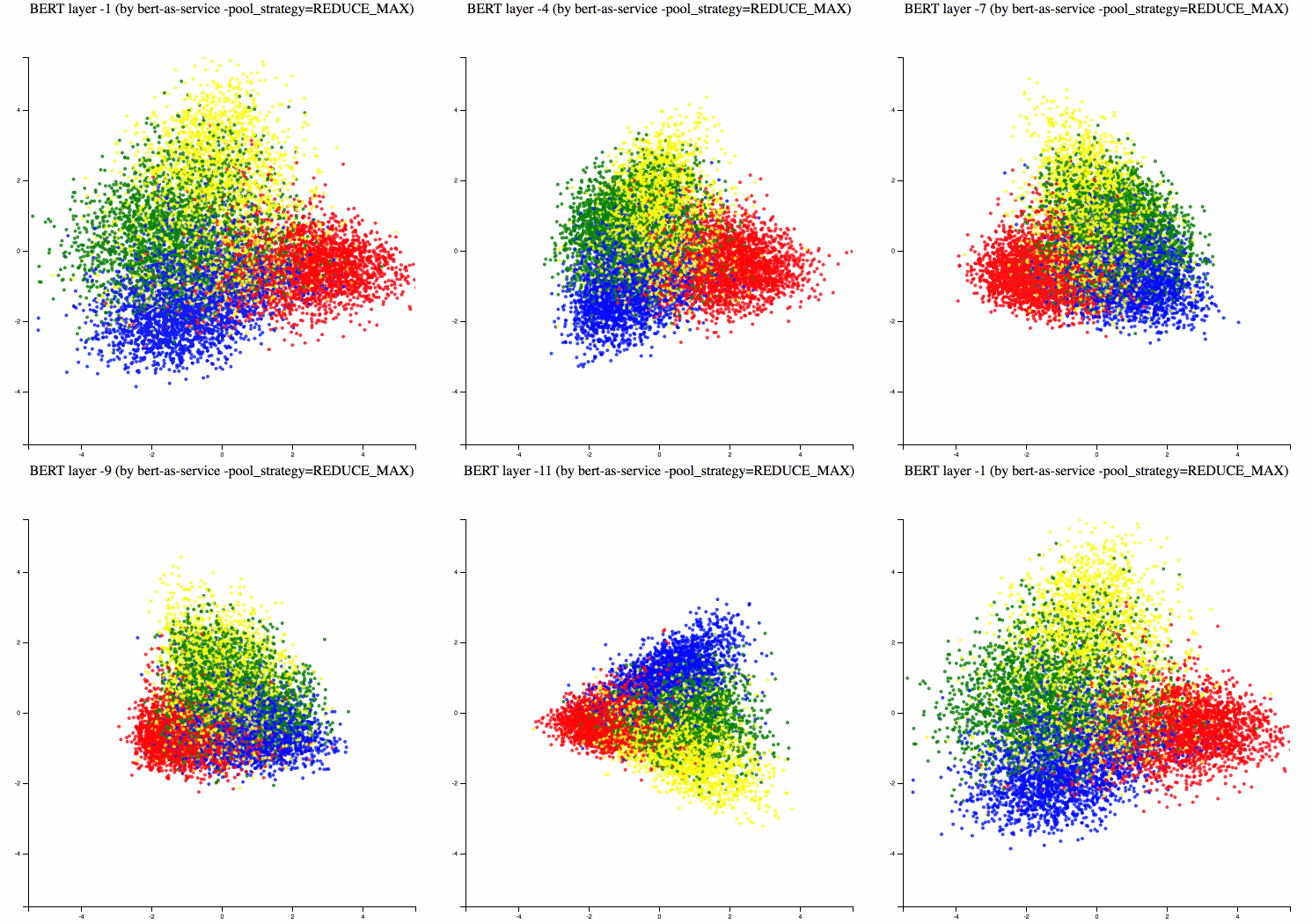
Different BERT layers capture different information. To see that more clearly, I made a visualization on UCI-News Aggregator Dataset with pretrained uncased_L-12_H-768_A-12, where I randomly sample 20K news titles; get sentence encodes from different layers using max and average pooling, finally reduce it to 2D via PCA. There are only four classes of the data, illustrated in red, blue, yellow and green.

One can observe that consecutive layers have similar representation, whereas the first few layers represent considerably different meaning compared to the last few layers. The deepest layer is the one next to the word embedding. It may preserve the very original word information (with no fancy self-attention etc.). On the other hand, one may achieve the very same performance by simply using word embedding. Therefore, anything in-between the first layer and the last layer is then a trade-off. The next animation illustrates the difference between layers more clearly.

Engineering: Building a Scalable Service

Fortunately, pooling is the only research problem that we have to face at the moment. The rest of the work is mostly about engineering.

Decoupling BERT and downstream network

The first thing to do is decoupling the main BERT model and the downstream network. More specifically, that 12/24-layer stacked multi-head attention network should be hosted in another process or even on another machine. For example, you can put it on a cost-per-use GPU machine, serving multiple teams simultaneously. The downstream network/models are often light-weighted and may not need deep learning libraries at all, they can run on a CPU machine or a mobile device.

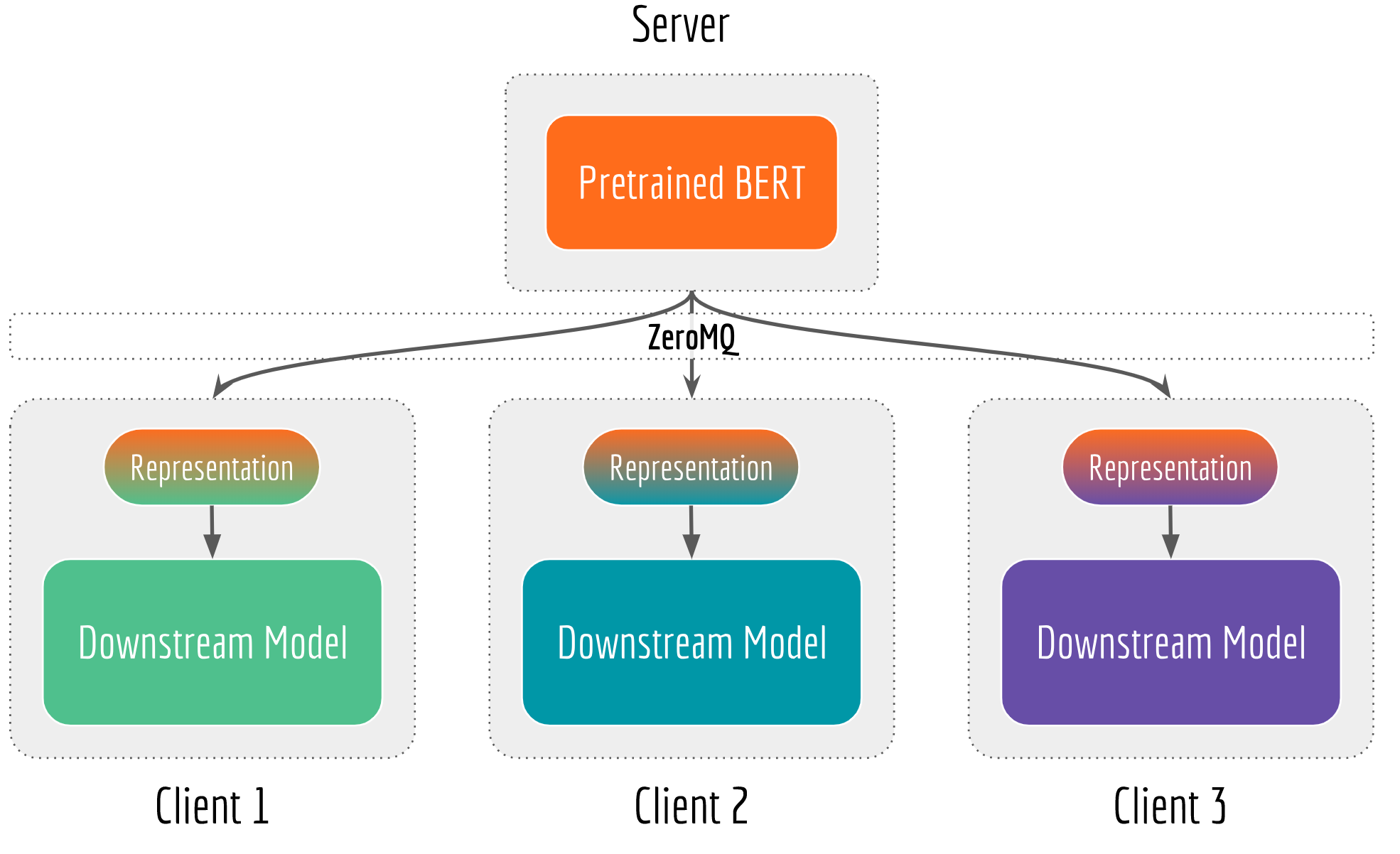
Decoupling also clarifies the C/S role. When the feature extraction becomes the bottleneck, then scale up the GPU server. When the downstream network is the bottleneck, then optimize the client by adding more CPU machines or doing quantization. When training data is too old or concept-drifted, then retrain the BERT and version-control the server, all downstream networks immediately enjoy the updated feature vectors. Finally, as all requests come to one place, your GPU server has less idle cycles and every penny is spent worthily.

To build the communication stack, I use ZeroMQ and its python bindings PyZMQ, which offer a lightweight and fast messaging implementation. You can send and receive an inter-process message via TCP/IPC/many other protocols simply as follows:

import zmq
import zmq.decorators as zmqd

@zmqd.socket(zmq.PUSH)
def send(sock):
    sock.bind('tcp://*:5555')
    sock.send(b'hello')
 
# in another process   
@zmqd.socket(zmq.PULL)
def recv(sock):
    sock.connect('tcp://localhost:5555')
    print(sock.recv())  # shows b'hello'

Serving with fast inference speed

The original BERT code released by Google supports training and evaluating. This introduces some auxiliary nodes that should be removed from the computational graph before serving. Also notice that if one uses the k-th layer for pooling, then all parameters from (k+1)-th to the last layers are not necessary for the inference and thus can be safely removed as well. The following picture summarizes a general procedure before serving a deep neural network in production.

Specifically, freezing substitutes all variables by constants, i.e. from tf.Variable to tf.Constant. Pruning removes all unnecessary nodes and edges from the graph. Quantizing replaces all parameters by their lower precision counterparts, e.g. from tf.float32 to tf.float16 or even tf.uint8. Currently, most quantization methods are implemented for mobile devices and therefore one may not observe significant speedup on X86 architectures.

Tensorflow provides APIs for freezing and pruning. We only need to specify the input and output nodes before optimizing the graph, such as:

input_tensors = [input_ids, input_mask, input_type_ids]
output_tensors = [pooled]

Then simply do:

from tensorflow.python.tools.optimize_for_inference_lib import optimize_for_inference
from tensorflow.graph_util import convert_variables_to_constants

# get graph
tmp_g = tf.get_default_graph().as_graph_def()

sess = tf.Session()
# load parameters then freeze
sess.run(tf.global_variables_initializer())
tmp_g = convert_variables_to_constants(sess, tmp_g, [n.name[:-2] for n in output_tensors])

# pruning
dtypes = [n.dtype for n in input_tensors]
tmp_g = optimize_for_inference(tmp_g, [n.name[:-2] for n in input_tensors],
    [n.name[:-2] for n in output_tensors],
    [dtype.as_datatype_enum for dtype in dtypes], False)
    
with tf.gfile.GFile('optimized.graph', 'wb') as f:
    f.write(tmp_g.SerializeToString())

Serving with low latency

We don’t want to spawn a new BERT model every time a new request comes in, instead, we want to spawn the model only one time in the beginning and listen to the request in an event-loop. Calling sess.run(feed_dict={...}) is one solution, but it’s not efficient enough. Besides, as the original BERT code is wrapped with high-level tf.Estimator API, we need to do some tweaks to inject the listener. A perfect place for such injection is in the generator of input_fn, which is the fundamental element of tf.Data API.

def input_fn_builder(sock):
    def gen():
        while True:
            # receive request
            client_id, raw_msg = sock.recv_multipart()
            msg = jsonapi.loads(raw_msg)
            tmp_f = convert_lst_to_features(msg)
            yield {'client_id': client_id,
                   'input_ids': [f.input_ids for f in tmp_f],
                   'input_mask': [f.input_mask for f in tmp_f],
                   'input_type_ids': [f.input_type_ids for f in tmp_f]}

    def input_fn():
        return (tf.data.Dataset.from_generator(gen,
            output_types={'input_ids': tf.int32, 'input_mask': tf.int32, 'input_type_ids': tf.int32, 'client_id': tf.string},
            output_shapes={'client_id': (), 'input_ids': (None, max_seq_len), 'input_mask': (None, max_seq_len),'input_type_ids': (None, max_seq_len)})
                .prefetch(10))
    return input_fn

Then, one can simply call:

# initialize BERT model once
estimator = Estimator(model_fn=bert_model_fn)
# keep listen and predict
for result in estimator.predict(input_fn_builder(client), yield_single_examples=False):
    send_back(result)

Note that estimator.predict() returns a generator and the above for-loop never ends. When there is a new request, the generator will prepare the data and feed it to the estimator. Otherwise, the generator will be blocked at sock.recv_multipart() until the next request.

Careful readers may notice .prefetch(10) at the end of tf.data.Dataset. Adding the prefetch mechanism can effectively hide the batch preparing time (on CPU, introduced by convert_lst_to_features()) behind the actual prediction time (on GPU). When the model is doing prediction and a new request comes in, no-prefetch will simply be blocked at yield until the prediction is finished, whereas with .prefetch(10) it will keep preparing batches until there are 10 pending batches queued for prediction. In practice, I found adding prefetch gives 10% speedup. Of course, this is only effective on a GPU machine.

There are other optimization tricks implemented in bert-as-service, including turn on XLA compiler. Interested readers are encouraged to read the source directly.

Serving with high scalability

Say multiple clients are sending requests to a server simultaneously. Parallelization on the computational work is one thing, but first, how should the server even handle receiving? Should it receive the first request, hold this connection until it sends back the result; then proceed to the second request? What happens if there are 100 clients? Should the server use the same logic to manage 100 connections?

As the second example, consider a client is sending 10K sentences at every 10ms. The server parallelizes the work into sub-tasks and assigns them to multiple GPU workers. Then another client joins in, sending one sentence per second. Instinctively, this small-batch-client should get the result instantly. Unfortunately, as all GPU workers are busy computing for and receiving from the first client, the second client will never get a time slot until the server finishes 100 batches (each with 10K sentences) from the first client.

These are scalability and load-balancing issues when multiple clients connect to one server. In bert-as-service, I implement a ventilator-worker-sink pipeline equipped with push/pull and publish/subscribe sockets. The ventilator acts like a batch scheduler and a load balancer. It partitions the large request from clients into mini-jobs. It balances the load of those mini-jobs before sending them to workers. The worker receives mini-jobs from the ventilator and does the actual BERT inference, finally sends the result to the sink. The sink collects the output of mini-jobs from all workers. It checks the completeness of all requests from the ventilator, publishes the complete results to clients.

The overall architecture is depicted below.

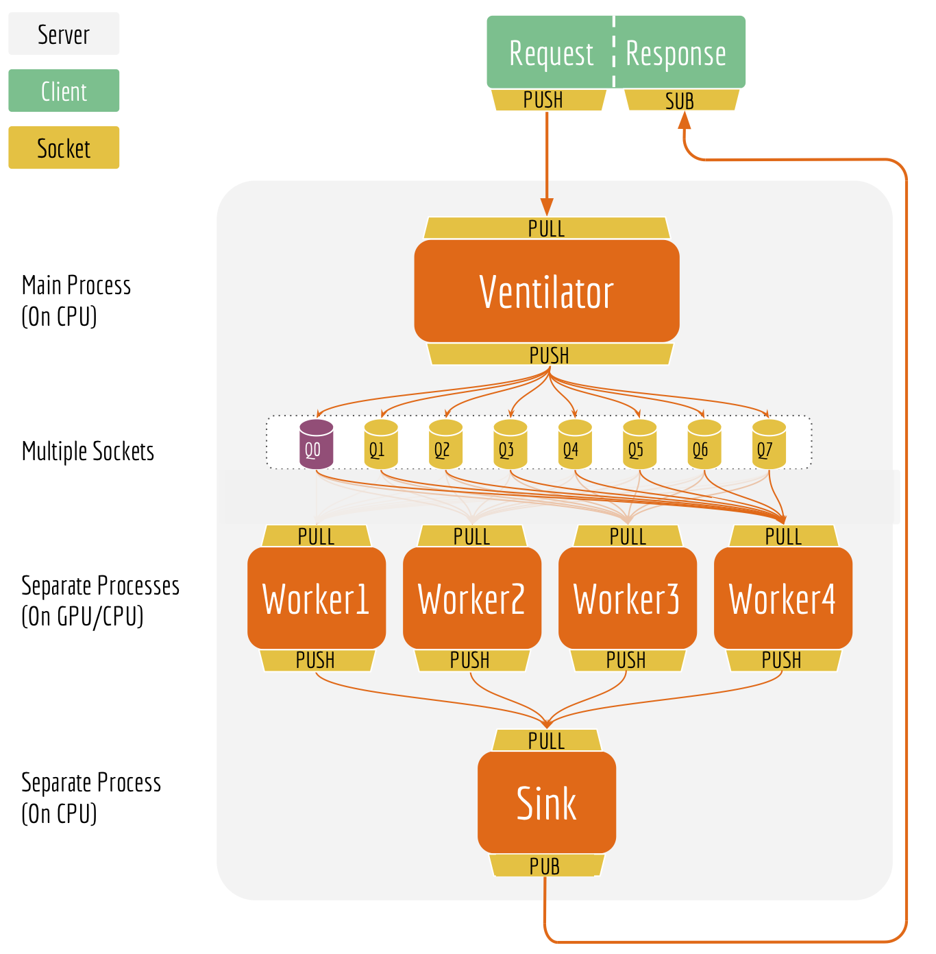
I have to confess this is not the first thing came to my mind. What you see here is the pipeline after multiple iterations, the one that very well solves the scalability issues mentioned above. Let me explain it in details.

• Separated sockets for send and receive on the client. Comparing to the standard REQ-REP socket (which is in lockstep), the PUSH-PULL socket does not wait for the response before the next PUSH. The client can send multiple requests in a row, then ask for the results later. When the computation is done, the server broadcasts the result via the PUB socket and uses client IDs as the header. The client listens to the broadcast from the SUB socket and fetches the subscriptions matching its own identity.

  There are at least two advantages of the PUSH-PULL and PUB-SUB design. First, there is no need to keep the connection alive between the server and the client. As a client, you just put the data to the predefined location, job’s done. You know someone (the server) will pick it up (via PULL). You don’t care about whether the server is alive or dead or restarted or parallelized. As the server, you go to the predefined location and get jobs. You don’t care about who put it there and how many are there. You do your best and load’em all! Same goes for receiving, every client gets its result from the predefined location as it knows that’s the place where results would appear. This design makes the system more scalable and robust. 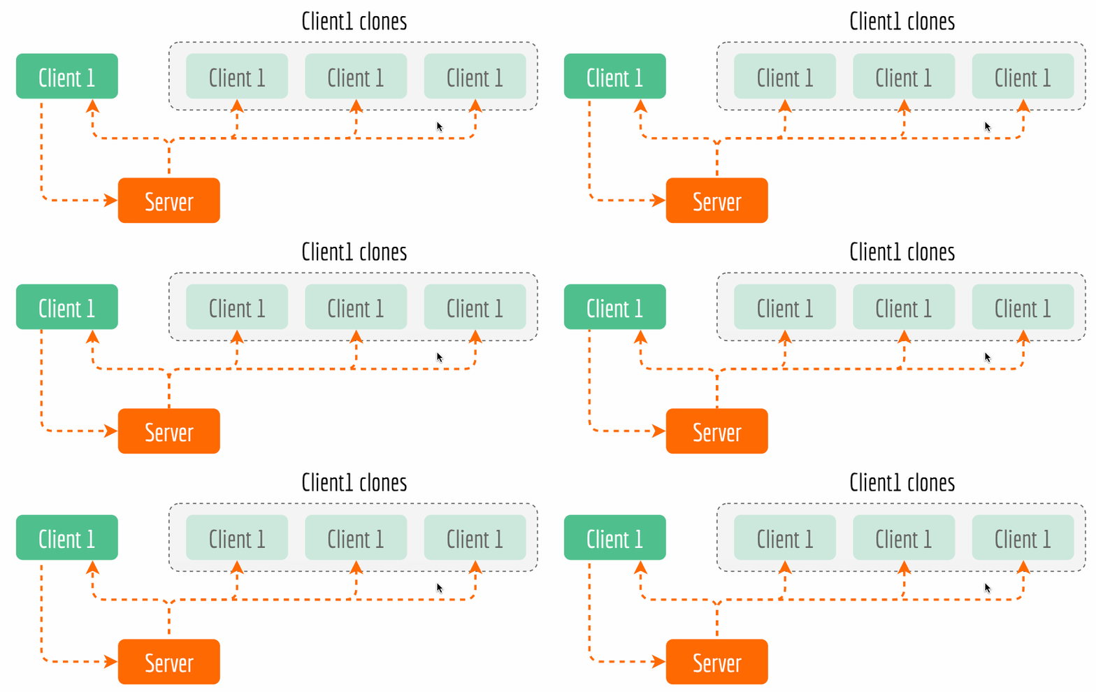In bert-as-service, you can simply kill the server and restart it, the same BertClient still works fine.

  The second advantage is that it enables cool features such as asynchronous encoding and multicasting. Async encoding is particularly useful when you want to overlap of sentence pre-processing time and the encoding time for efficiency reasons. Now multicasting is a part of BertClient API, which allows multiple clients with the same identity to receive the results simultaneously while only encoding once. The next figure illustrates this idea. The complete example can be found here.

  

• Kill back-chatters. Careful readers may notice that data always flows down the pipeline: all messages are not sent upstream but only sent downstream to another socket, and the recipients don’t talk back to senders. Killing back-chatter is essential to real scalability. When we remove back-chatter, the overall message flow becomes much simpler and non-blocking, which lets us make simpler APIs and protocols, and in general lower latency.

• Multiple sockets between the ventilator and workers. If the size of a request is smaller than 16 sentences, then the ventilator pushes the job to the first socket (Q0 in the architecture graph). Otherwise, the ventilator partitions the job into mini-jobs where each has at most 256 sentences, then push these mini-jobs to a random socket from 1 to 7. The workers keep pulling jobs from all eight sockets following the ascending index order.

  This ensures that the small request won’t be blocked by the large-and-high-frequency request. A small request always goes to Q0, which gets pulled by the workers first. For large-and-high-frequency requests from multiple clients, they will be pushed to different sockets and get an equal chance for computing on the workers.

• Separated processes for the ventilator, workers and the sink. Separating components at the process-level improves the robustness and reduces the latency. One may argue that the sink and the ventilator can be combined into one module. But then a result message would still have to travel across process, which won’t reduce the communication cost. Besides, having separated processes keeps the overall logic and message flow simple. Every component focuses on one job only. We can easily scale up the sink or the ventilator when either becomes the bottleneck.

Finally, interested readers are always welcome to read the source directly. To validate the efficiency of this architecture, I benchmarked the service with different parameters, achieving ~900 sentences/s on single GPU and scaling nicely on multi-GPU or with multi-client. The full result can be found in the last section of the Github README.md.

Summary

Since the release of bert-as-service in Nov. 2018, it has received quite some attention from the community. It collected more than 1K Github stars in a month. People message me and appreciate for its simplicity and scalability, allowing them to quickly try the latest NLP technique. Personally, deploying a deep learning model into production is always a great learning experience. As written in this post, it requires knowledge on both research and engineering sides to make things really work. I also greatly appreciate the community for pointing out bugs, improvements and new ideas. There was indeed some busy days. But these feedbacks eventually bring the quality of the project to the next level. Having a deep learning model in production is more than a lesson, especially when it starts to receive real traffic. You can simply lay down on the chair, watch the dashboard pulsing back and forth, and enjoy this great accomplishment for the rest of the day.