4 Sequence Encoding Blocks You Must Know Besides RNN/LSTM in Tensorflow
Background
Understanding human language is a challenging task for computers, as they were originally designed for crunching numbers. To let computers comprehend text as humans do, one needs to encode the complexities and nuances of natural language into numbers. For many years, recurrent neural networks (RNN) or long-short term memory (LSTM) was the way to solve sequence encoding problem. They have indeed accomplished amazing results in many applications, e.g. machine translation and voice recognition. As for me, they were the first solution that comes to my mind when facing an NLP problem. You can find my previous posts about RNN/LSTM in here, here, and here.
Now at Tencent AI Lab, however, I’m sunsetting RNN/LSTM in my team. Why? Because they are computationally expensive, aka slow! The recursive nature requires it to maintain a hidden state of the entire past that prevents parallel computation within a sequence. Also, don’t forget that sequence encoding is often just a low-level subtask of our ultimate goal (e.g. translation, question-answering). The upper layers are waiting for the encodes so that they can carry on more interesting tasks. Thus, it is not worth spending so much time on the encoding task itself.
All in all, we need our sequence encoding to be fast. A faster sequence encoder boosts the development cycle of our team, enabling us to find the optimal model by exploring more architectures and hyperparameters, which is crucial for bringing AI into production.
In this article, I will introduce four sequence encoding blocks as a replacement of RNN/LSTM. I’d like to call them “block”, as they all consist of multiple layers or even other blocks. They can be further nested, duplicated or joined to compose a more power super-block, improving a network’s capacity and expressivity.
The code mentioned in this post can be found on my Github. Readers are welcome to contribute or give suggestions.
Table of Content
- What is a Sequence Encoding Block
- Pooling Block
- CNN Block
- Multi-Resolution CNN Block
- Multi-Head Multi-Resolution CNN Block
- Summary
What is a Sequence Encoding Block
As you may find people referring the encoding task differently, such as fusing, composing and aggregating. I’d like to first clarify the definition of an encoding block, so we are on the same page.
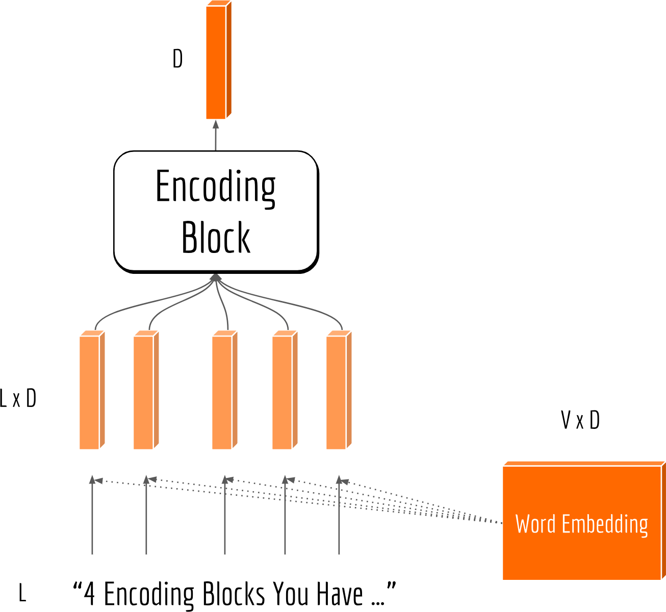
Considering a text sequence (e.g. a sentence, a paragraph, a document) represented as $\mathbf{s}:=\{w_1, w_2, \ldots, w_L\,|\,w_l \in \mathcal{V}\}$, where $w$ denotes a word from the vocabulary $\mathcal{V}$ and $L$ denotes the length of the sequence. Let $\mathbf{M}$ be a word embedding matrix of size $|\mathcal{V}|\times D$, each row represents a word in $\mathbb{R}^D$. The word embedding matrix $\mathbf{M}$ can be obtained with GloVe or Word2Vec, or be initialized randomly and learned from scratch. Either way, one can now represent $\mathbf{s}$ as a $L\times D$ matrix via tf.embedding_lookup on $\mathbf{M}$. The goal of a sequence encoding block is to find a function $\mathbb{R}^{L\times D}\rightarrow\mathbb{R}^{D^\prime}$, which encodes information of a variable length sentence into a fixed-length vector representation. The $D^\prime$-dimensional output vector is then fed to the upper layers for the final task. The next figure illustrates this idea.
Pooling Block
Average Pooling and Max Pooling
Let’s start with the simplest ones: reducing the dimension $L$ to 1 by taking the average/maximum over each of the $D$ dimensions. They can be (almost) easily implemented tf.reduce_mean and tf.reduce_max, respectively. I say almost, as one has to be careful with the padded symbols when dealing with a batch of sequences of different lengths. Those paddings should never be involved in the calculation. Tiny details, yet people often forget about them.
These two strategies are also called average pooling and max pooling, respectively. Both of them make perfect sense intuitively: in average pooling the meaning of a sentence is represented by all words contained; whereas in max pooling the meaning is represented by a small number of keywords and their salient features only.
Hierarchical Pooling
To keep the best part of two sides, one can combine these two strategies together: via concatenating, i.e. tf.concat, or hierarchical pooling. In hierarchical pooling, we first define a small sliding window. The window moves across the dimension $L$. Then we do reduce_mean at every move and collect the result, finally do reduce_max on all results. Here I show a Tensorflow implementation of the hierarchical pooling strategy:
1 | def reshape_seqs(x, avg_window_size=3, **kwargs): |
The trick here is to reshape the batch sequence in advance from the shape [B,L,D] to [B,D,W,L'/W], where W is the size of the sliding window, and L' is the length with extra paddings so that it can be divided by W. As a consequence, one can simply apply average pooling on the third dimension followed by a max pooling on the last dimension. Just be careful with padded symbols and the mask.
Comparing to max and average pooling, hierarchical pooling captures more local spatial information because of the preservation of the word-order in each window. The size of the window is a trade-off between the max and average pooling. One may also relate it with bag-of-n-grams described in this paper.
Attentive Pooling
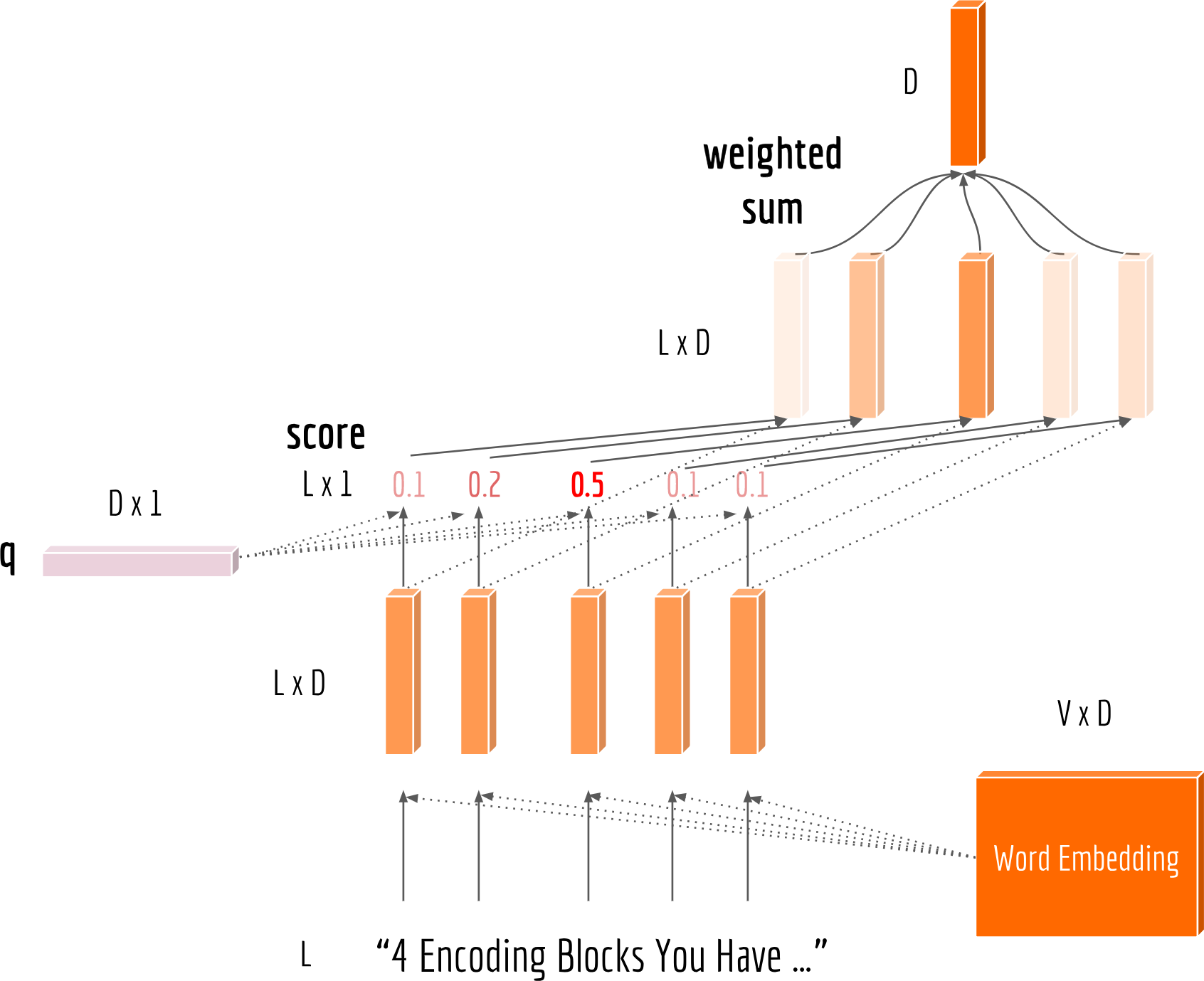
We can also let the model automatically pick up the important words to represent a sentence. One solution is attentive pooling. Specifically, I introduce a $D$-dimensional global variable $\mathbf{q}$. We first multiply the sequence with $\mathbf{q}$ and get a “score” of length $L$. Each element of the score represents the importance of a word to the sequence. Finally, a weighted sum is conducted over all words according to the score. The figure below illustrates the attention procedure.
The code is simple as follows:1
2
3
4
5B = tf.shape(seqs)[0]
D = tf.shape(seqs)[-1]
query = tf.tile(get_var('query', shape=[1, D, 1]), [B, 1, 1])
score = tf.nn.softmax(minus_mask(tf.matmul(seqs, query) / (D ** 0.5), mask), axis=1) # [B,L,1]
pooled = tf.reduce_sum(score * seqs, axis=1) # [B, D]
Again, the mask and padded symbols need to be taken care of before computing softmax. This can be done by subtracting a large number using minus_mask. Besides the scaled matrix multiplication mentioned above, there are other attention functions. Interested readers are recommended to read Sect. 4.3 in this paper.
Final Touch
As our first block, I don’t want to make it too complicated. So let’s finish it with some final touch. Here I add layer normalization and dropout to improve the robustness and generalization ability. Finally, a complete pooling block looks like the following:
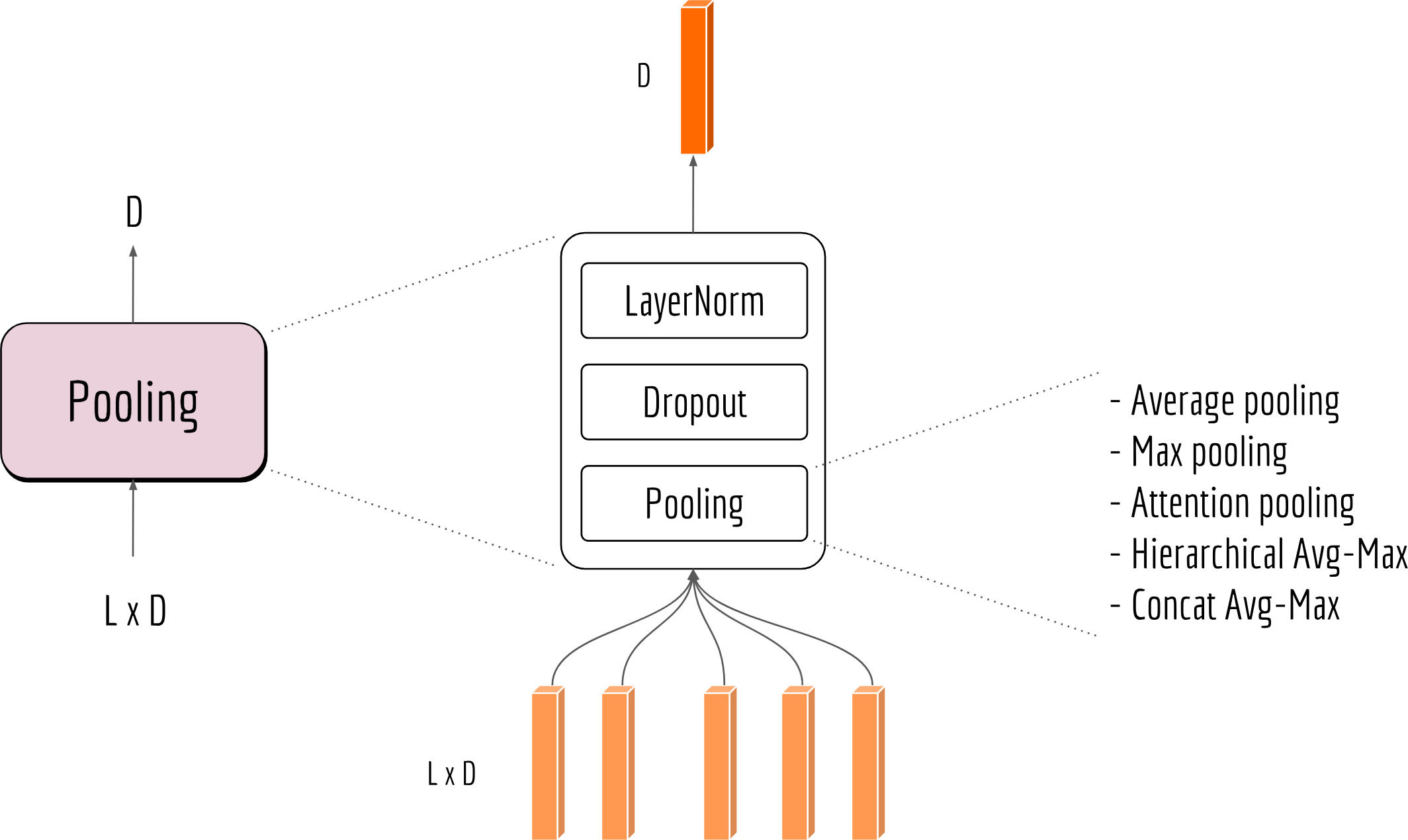
As we shall see later, the pooling block is a cornerstone for more sophisticated encoding blocks.
CNN Block
There has been excellent work with CNNs on NLP before, as in “Natural Language Processing (almost) from Scratch”. The basic idea is to use a 1-D kernel with a small width and slide it over the entire sequence. In some sense, this idea is very similar to the hierarchical pooling as I described in the last section. The major difference is that CNN’s kernel is not a simple average: it is parameterized and needs to be learned from the data. The code below describes how to apply convolution on a sequence:1
2
3
4
5seq_dim = seqs.get_shape().as_list()[-1]
W = get_var('conv_W', [kernel_width, seq_dim, num_filters])
b = get_var('conv_bias', [num_filters])
conv = tf.nn.conv1d(seqs, W, stride=1, padding='SAME')
output = tf.nn.relu(tf.nn.bias_add(conv, b))
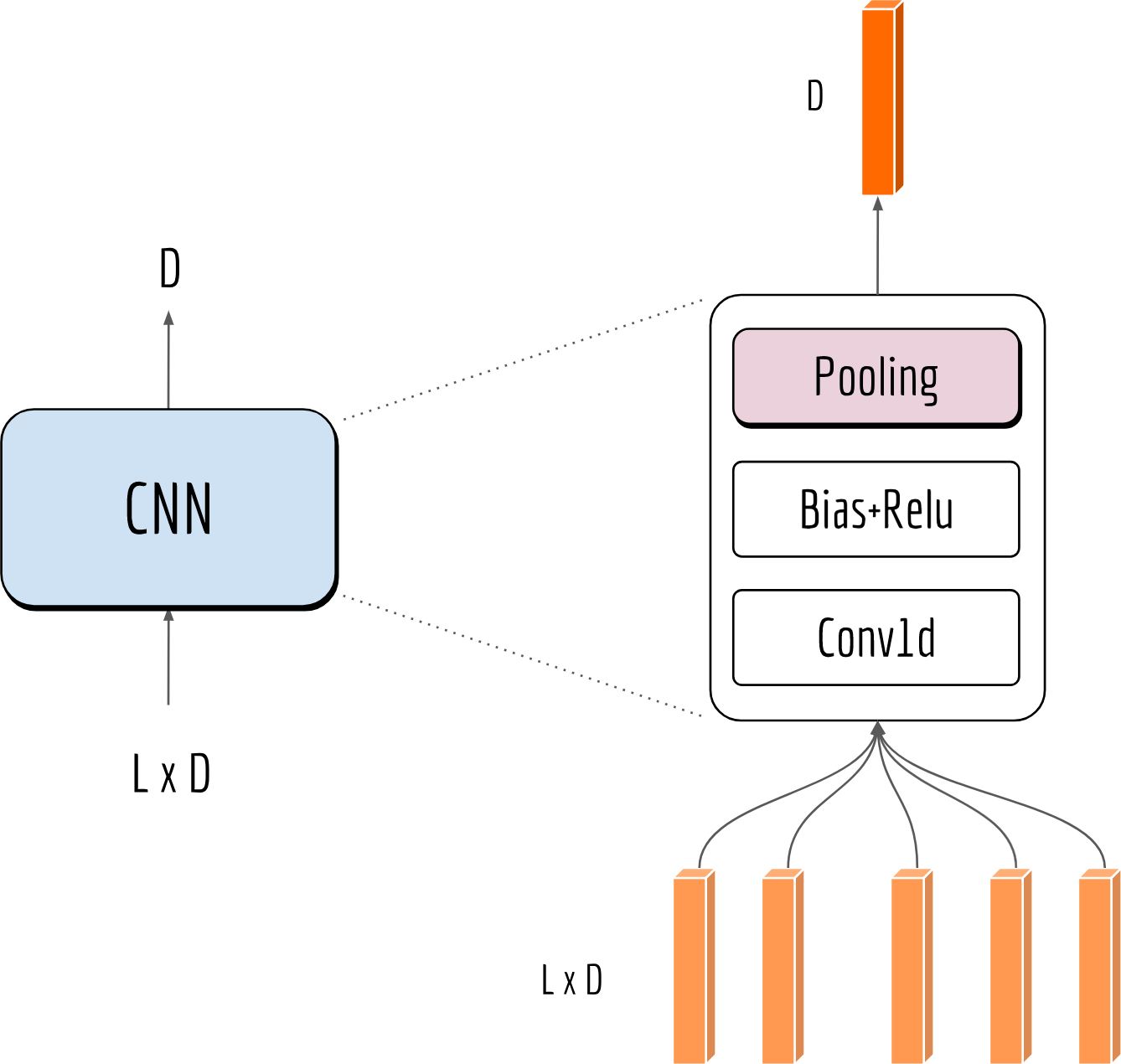
Note that the output has the shape [L, D] when using padding='SAME', meaning the full input sequence length $L$ is retained. To introduce some non-linearities, I add a bias to it and wrap it with a ReLU activation function. One may also understand it as a “gate”, keeping only the salient values for the output. Finally, the output is fed to a pooling block for transforming it into a fixed-length vector. The next figure illustrates this process:
Causal Convolutions
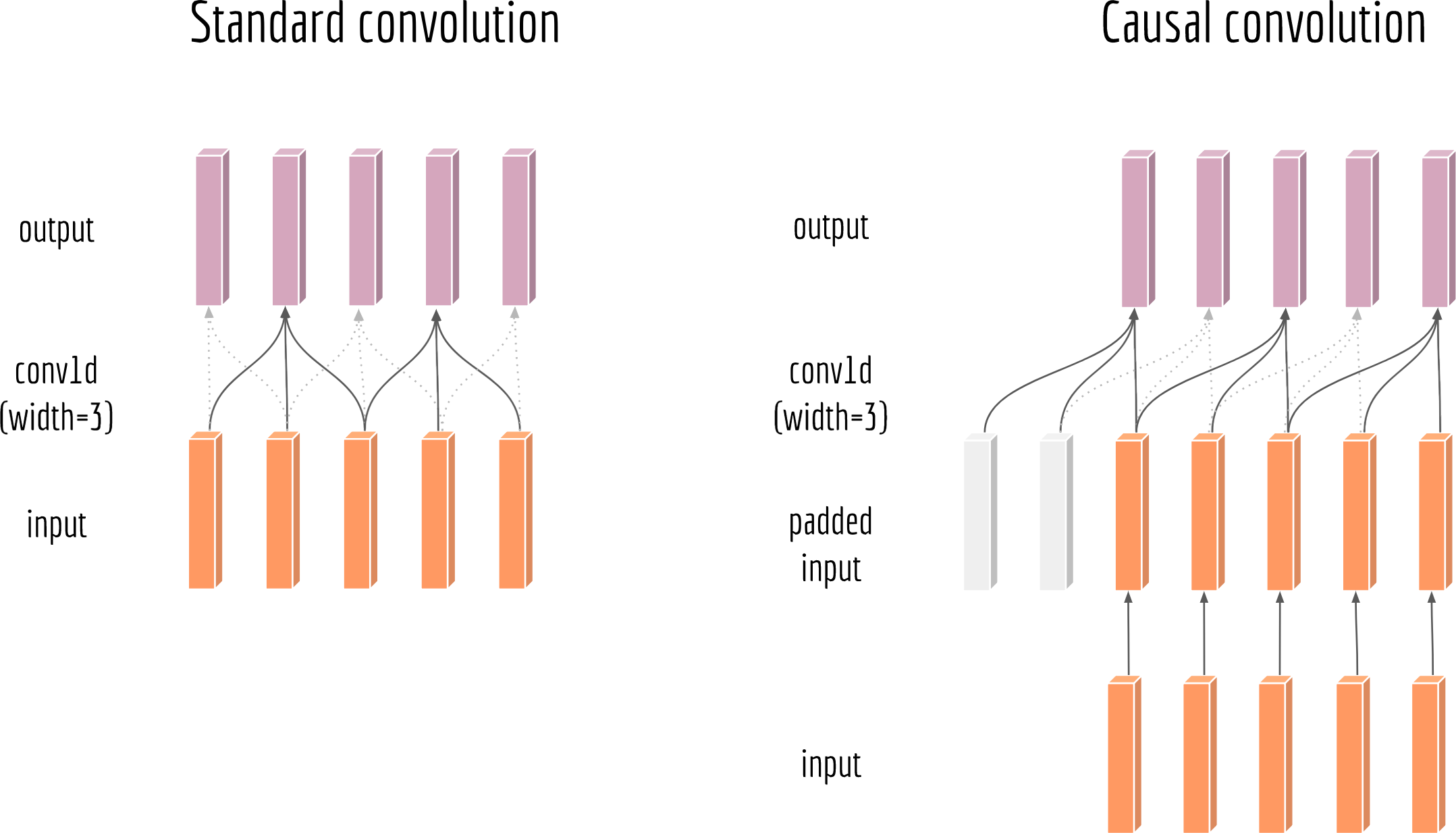
One may argue that the above CNN block is cheating as it leverages the future information. To make it clear, assuming we have a block with kernel_width=3 then the convoluted output of time $l$ depends on the input of $l-1$, $l$ and $l+1$. This is different than standard RNN/LSTM, where each step $l$ only depends on the past ($\leq l$) not on the future.
To make it more RNN/LSTM-like, I introduce causal convolutions, in which an output at time $l$ is convolved only with elements from time $l$ and earlier in the input. This can be simply done by padding kernel_width -1 empty symbols to the left of the sequence. The next figure illustrates this idea vs. the standard convolution.
The code is simply as follows:
1 | padding = (kernel_width - 1) |
Shifting the sequence to change time-dependency of the model is nothing new. It is essentially the same tweak as described in the time delay neural network proposed nearly 30 years ago.
Multi-Resolution CNN Block
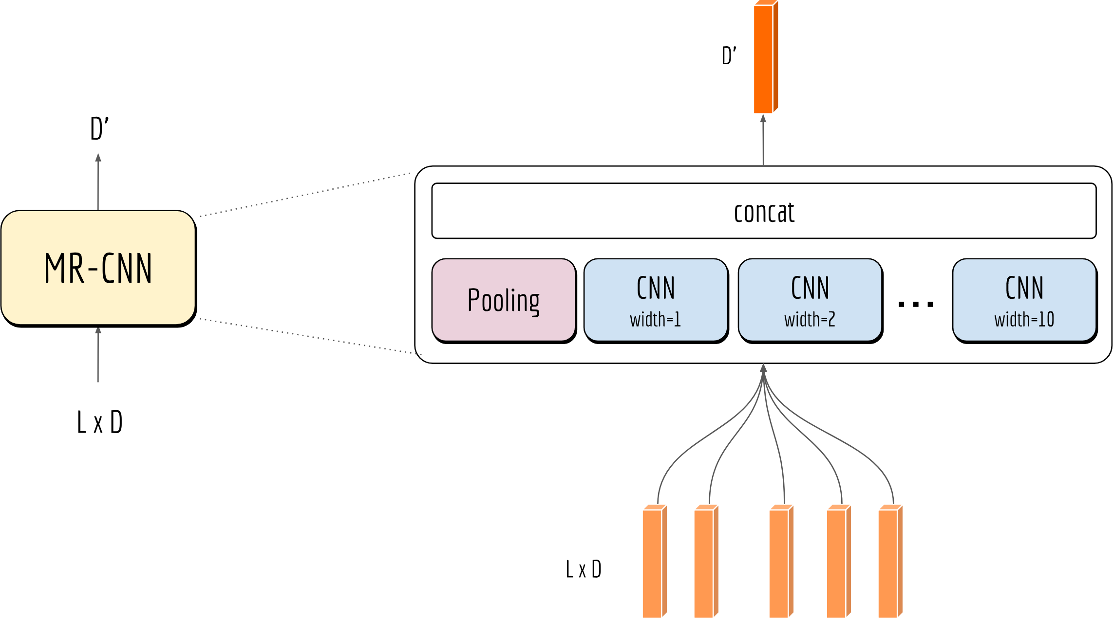
The hyperparameter kernel_width controls the resolution of the CNN block. When applying it on a sequence, kernel_width corresponds to the context size $n$ of n-gram. An ideal kernel width is important but also task-dependent. As a workaround, one can simply employ multiple CNN blocks with different kernel widths and concatenate their outputs together. The code is presented below:1
2
3
4outputs = [Pool_Block(seqs, mask, **kwargs)] if highway else []
for fw in kernel_widths:
outputs.append(CNN_Block(seqs, mask, fw, scope='cnn_%d' % fw, **kwargs))
output = tf.concat(outputs, axis=1)
Note that I let the input bypass all CNN blocks when highway=True. This shortcut is particularly useful when training a very deep network, as the gradient can be propagated back to the low-level layers more easily through this highway. The next figure visualizes this block:
One may also stack CNN blocks on top of each other to increase the context size. For instance, stacking 5 CNN blocks with kernel width of 3 results in an input field of 11 words, i.e., each output depends on 11 input words. Personally, I found such deep encoders are more difficult to train well in practice, and its improvement on NLP tasks is marginal. But who am I to say that?
Multi-Head Multi-Resolution CNN Block
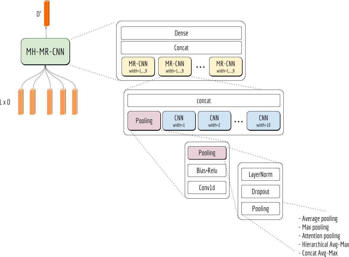
The term “multi-head” comes from Google’s paper Attention is All You Need, where it stacks multiple attention bocks for a single input and creates a powerful but fast-to-train model. The parameters of those attention blocks are not shared. The expectation is that each “head” can capture a unique aspect of the sequence, thus together they can improve the expressivity of the model.
Inspired by this idea, here I stack multiple MR-CNN blocks to build a multi-head multi-resolution CNN block. A fully expanded view of this block is depicted in the next figure. A global highway is probably not necessary here as each MR-CNN block already has its own highway.
Implementation Trick
While we keep stacking and nesting blocks into one, the number of hyperparameters keeps increasing. This also means the function identifier contains quite some arguments. Take a MH-MR-CNN block as an example,
1 | encode = MH_MR_CNN(seq, mask, |
Note that most of the arguments are not for MH-MR-CNN except num_heads. Nonetheless, they still need to be carried all the way back to the deepest block, i.e. the pooling block. A naive way to implement this is writing all hyperparameters in all function identifiers, passing them via explicit function arguments. A better way is to use **kwargs, a Python feature which allows you to pass a variable number of arguments to a function. If a function can’t handle some of those arguments, then you can simply forward **kwargs to its sub-functions, etc. The code below demonstrates this trick:
1 | def Pool(seqs, mask, reduce='concat_mean_max', norm_by_layer=False, dropout_keep=1., **kwargs): |
As one can see, by using **kwargs each block only declares its own hyperparameters in the function identifier, resulting in a much cleaner and more readable code.
Summary
A sequence encoder is the cornerstone of many advanced AI applications, such as semantic search, question-answering, machine reading comprehension. Therefore, how to encode sequences good and fast is considered as a fundamental problem in the ML/NLP community. In this post, I have introduced four non-RNN encoding blocks which are extremely useful in practice. In some NLP task where long-term dependencies are not so important (e.g. classification), those non-RNN encoding blocks can perform competitively to recurrent alternatives and save you a lot of computational time.
The code mentioned in this post can be found on my Github.